2 Data for environmental science
What do electrons, molecules, quarks, DNA, addition, subtraction have in common? They each may be considered the fundamental building blocks for physics, biology, chemistry, and mathematics (Marth 2008). For environmental data science, the fundamental building block is contained in the name itself: data. Setting aside the broader discussion of how data happened (Wiggins and Jones 2023), this chapter introduces formats in which environmental data mqy appear. Through examples, we will also discuss ways in which data can be imported into a local computing environment for analysis. Let’s begin.
2.1 Data tables and flat files
Environmental data are frequently presented in tables, which often represent values of an observed quantity. One such example is Figure 2.1, which is a screenshot from a long-term dataset of daily weather observations (going back to 1871!) recorded at a Minneapolis and Saint Paul International Airport in Minnesota.
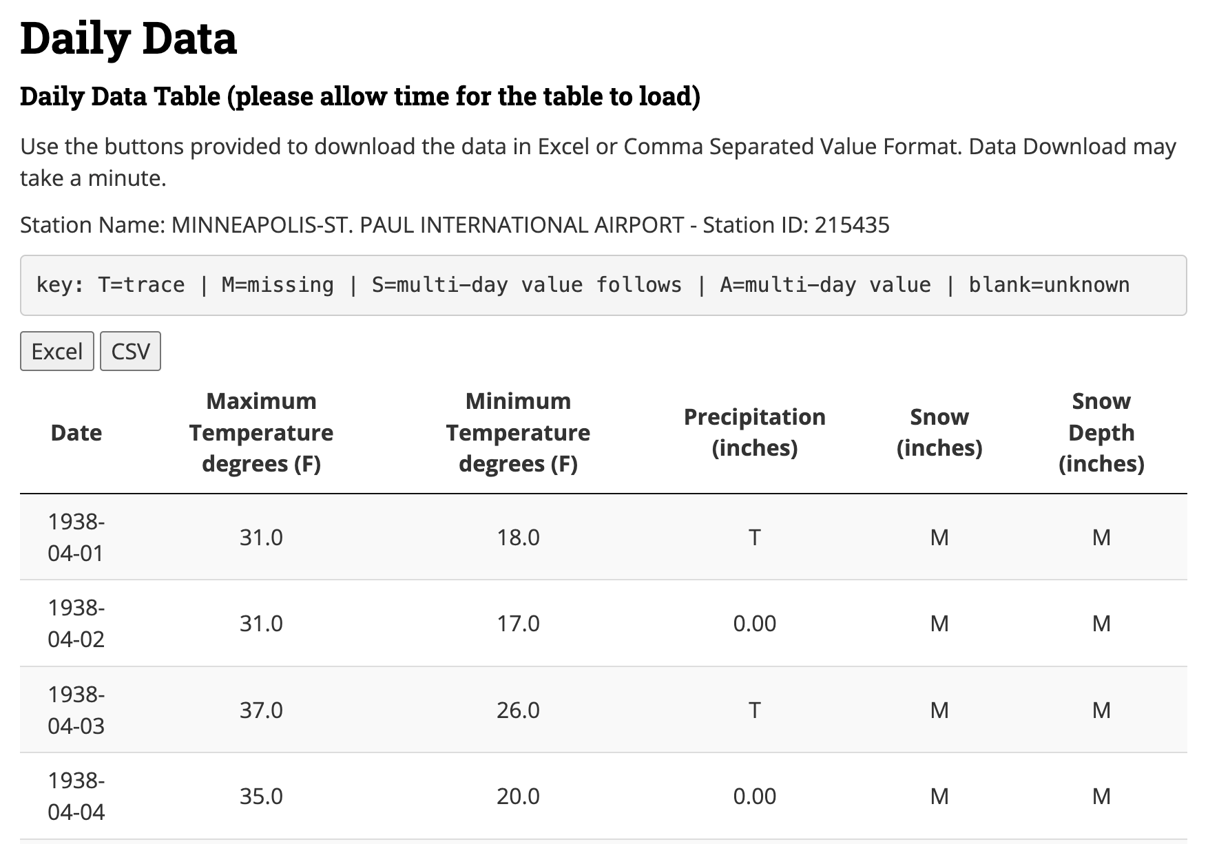
Figure 2.1 is a good starting off point illustrating the different types of data that can be found with environmental science. Once the data are imported into a statistical software program you are ready to use this information for other data transformations or statistical analyses. The first column Date represents a timeseries variable, and the remaining columns (e.g. maximum temperature, minimum temperature, precipitation, snow, and snow depth) generally represent quantitative variables. However the provided key in Figure 2.1 also notes that variables may have coded text values - “M” for missing or “T” for trace amounts in the table preview.
The data in Figure 2.1 can also be downloaded as a comma separated values (csv) file or an Microsoft Excel (XLSX) file. These files can then be used in programs such as Google sheets or Microsoft Excel. Both file types (CSV or XLSX) are examples of flat files or spreadsheets. Flat files prescribe an organizational structure of two dimensions - each column is a variable and every row a set of observations. Another name to qualify the data table in Figure 2.1 is tidy - which is explored more in Chapter 6. Most time, tidy data is easily imported into a software program with minimal effort.
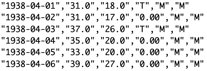
Comma separated value files rely on delimiters, which indicate different variables for an observation. Figure 2.2 displays the actual content of the CSV file associated with Figure 2.1, which can also be opened with a plain text file.1. Each row in Figure 2.2 corresponds to a day, or an observation of the weather. The presence of a comma instructs the computer to switch to the next variable in the table. Because commas are sometimes used to denote a decimal place, a CSV file may also use semicolons (;) as a delimiter. Other common delimiters may include tabs or spaces. The file extension “CSV” may be exclusively reserved to comma or semicolon delimiters, but tabs or spaces may have the extension of “TXT”.
Excel spreadsheets (.xlsx or the older .xls extension) are not considered flat files because they contain additional information about individual cell formatting and other information. The good news is that most statistical software programs can read in these files, but may require loading some additional packages / libraries in order to do so (i.e. readxl for R or openpyxl in Python).
Importing a CSV file into a statistical software program have special functions that systematically, quickly, and efficiently import the information line by line into a data table for analysis. Both R and python have functions named read_csv (tidyverse R and pandas Python) or read.csv (base R). For example, when we saved this data file and imported it into R using read_csv we have the following output in Figure 2.3:
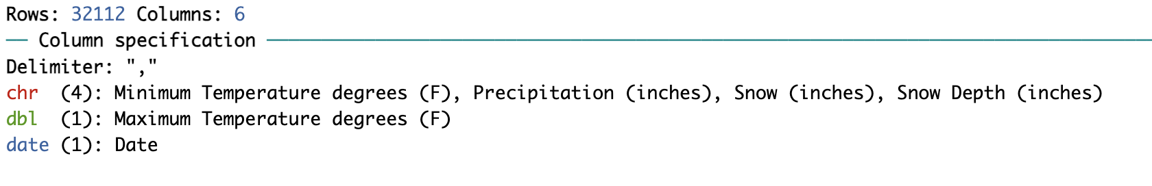
read_csv function to read in a comma separated values (csv) file.
A key thing to note in Figure 2.3 is the text below the variable name (date or chr) which specify the type of data that is read by the program. Other common types of data include:
- characters: ‘a’, or “2” (usually enclosed in a single or double quotes)
- integer: -3,-2,-1,0,1,2,3 …
- numeric: decimal numbers (3.25, 2.71, etc)
- binary: TRUE or FALSE
- dates: timeseries data
Notice that the variable starting with Maximum Temperature in Figure 2.3 has a data type of <chr>, but in reality, the data type should be numeric. The reason for this is the presence of the character M (see Figures 2.1 and 2.2). The function used to read in the flat file automatically assumes that any column containing a mixture of characters and numeric information is automatically a character. It is up to you to determine how best to modify and mutate these data (should we just exclude these measurements, set them to 0?). This is where you begin to exercise a modicum of choice and control in a data scientist, which will undoubtedly have implications for your analysis.
If you decide to change or modify data to make it conform to numeric or quantitative data (such as changing trace measurements to zero), be sure to document your assumptions in your workflow.
2.1.1 Common data structures
If data are the building blocks, there is a hierarchy of data structures and organization up to a spreadsheet or a flat file:
- Scalars are a single data value, which may include the data types listed above.
- Vectors are a collection of data of the same type. In the examples that we have examined, “Date”, “Temperature” (a single variable) would be the outputs.
- Data frames are a structured set of vectors of the same dimension, but may include vectors of different types. A flat file read into a spreadsheet program could be considered a data frame.
A final data structure is a list, which is a collection of scalars, vectors, or data frames. I think of these as a grab bag of items.
2.1.2 Working with dates
Dates and timeseries in files are often initially read into computational programs as strings, and thus need to be converted if any computation or mathematics needs to be computed. For example, consider the following questions:
- What day of the year is June 13, 2023? (1st, 2nd, 3rd, … )
- What day of the year is June 13, 2024?
- What day of the year is June 13, 2020?
- What week of the year is June 13, 2024?
- What day of the week is June 13, 2024? (1st, 2nd, 3rd, … ) or (Sunday, Monday, Tuesday …. )
- What hour of the day (out of 24) is 1:00 PM?
- At 1:00 PM, what percentage of the day has passed?
Can you answer the following questions on pencil and paper? Congratulations if you can, but questions like these can be a challenge for most people.2
To help ease some of the computational challenges that occur (accounting for leap years, daylight savings time, etc), the lubridate package in R provides easy interfaces to work with time objects. For more information about handling dates, see Chapter 17 in Wickham and Grolemund (2017). Equivalent packages in Python include datetime or dateutil.
A working knowledge of handling dates is important especially when comparing multiple geographic sites that may not be proximate to each other. The National Ecological Observatory Network (NEON) uses UTC as a timestamp for easy comparison, across sites, although other data repositories may just report the local time.
It is worth investigating the available options when working with timeseries data - lubridate for example provides functions to extract out any particular time component of a date object, or also computation of intervals between two dates.
2.2 More complex data tables
We argue flat files may be the easiest types of data files to import into a software program, but sometimes structured files contain extra information before they can be read into a program. Figure 2.4 is a plot of annual streamflow data from the Mississippi River in Saint Paul, Minnesota (USGS Geological Survey, n.d.).
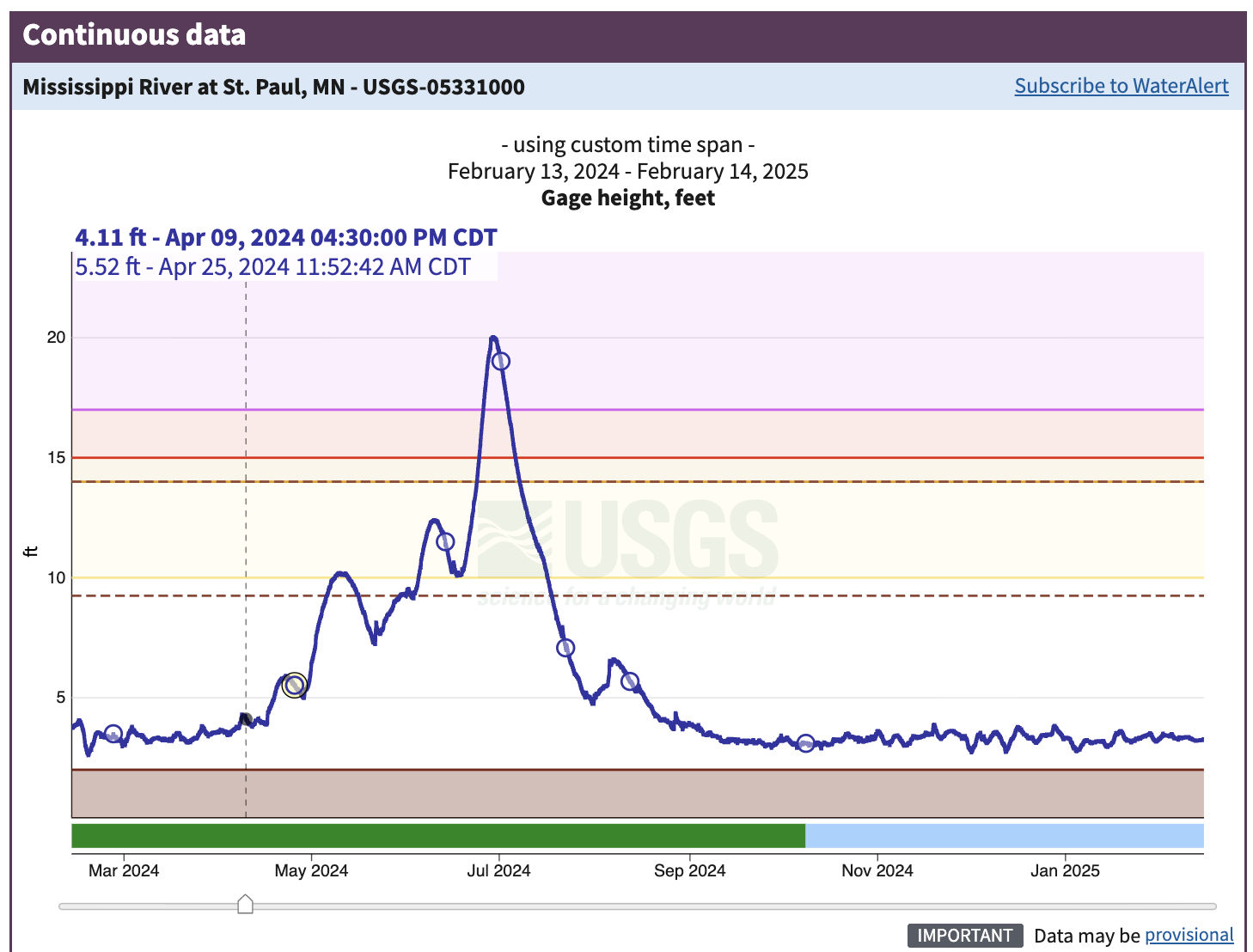
The data in Figure 2.4 highlight about the dynamic nature of a river in an urban environment. The coloring on the graph indicated different levels of flood stages:
- 10 - 14 feet (yellow): Action stage
- 14 - 15 feet (orange): Minor flood stage
- 15 - 17 feet (red): Moderate flood stage
- Greater than 17 feet (purple): Major flood stage
The rapid increase and decrease in the gage height over the course of the year indicates pulses due to rain events (May to July 2024), which was an exceptionally wet time in Minnesota.
Figure 2.5 displays a screenshot of the file structure as displayed in a text editor.
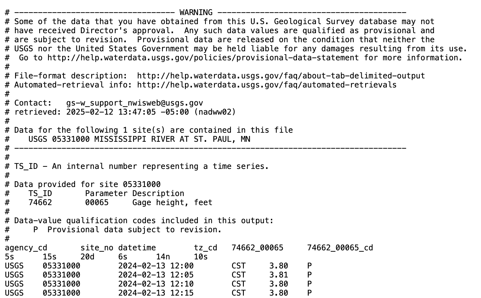
This information shown in Figure 2.5 looks different from Figure 2.2. The first few lines prefaced by a hashtag (#) denote header information - which could indicate how the data originated or its provenance, along with other notes and information. We need to make sure that any program that attempts to load this file ignores all the lines that start with the hashtag. Using a text editor, direct inspection of the lines that follow the hashtags suggests the tab (\t) as a possible delimiter. For this file we can’t use read_csv because this is a text file. In R, the function read_tsv allows for easy reading, using the option comment = “#” to ignore the whitespace.3 Python pandas does not have read_tsv, but read_csv with the delimiter \t.
It is always worthwhile to inspect the file in a text editor first to see if there is additional header information.
2.3 Moving to larger open-access datasets
Chapter 2 is an entry point to some of the types of data files you may encounter in environmental data science. Datasets could be maintained in distributed code libraries. For example, there are upwards of 2300 datasets available for use in the R software program (see Rdatasets) and R packages (which may also contained datasets) maintained by CRAN also approximate 20000 (Hornik et al. 2023).
A major consideration is the size of flat files, which is a practical limitation to read these into a software program. Chapters 6 - 8 will introduce you to other types of complex data structures (e.g. hdf files, videos, sounds) as tabular data under the hood. These datasets can be analyzed with many computational programs, but the bottleneck requires the ability to incorporate them into your computational program, or what we term in Chapter 3 as the computational environment.
2.4 Exercises
Inventory the types of data that you may use in your research. Are they timeseries data? Categorical data? Repeated measurements? How are the data structured? What programs do you use to analyze these data?
Using either R or Python, explore the various functionalities to read data into your favorite software program. How would you specify comments? Are there tools for date conversions?
The data table in Figures 2.1 and 2.2 for Section 2.1 converted all columns with a mixture of characters and quantitative information as characters. Let’s explore what would happen if we were to force a character strings to be numeric:
- Using R, what is the output of this statement:
as.numeric(c(4,"3","Q"))? - Using Python, what is the output of this statement:
pandas.to_numeric([4, "3", "Q"])? - Using Python, what is the output of this statement:
pandas.to_numeric([4, "3", "Q"], errors="coerce")?
- Using R, what is the output of this statement:
Explain the differences between each of the outputs for the different software languages.
Use
lubridatein R ordatetimeordateutilin Python to answer the following questions about dates:- What day of the year is June 13, 2023? (1st, 2nd, 3rd, … )
- What day of the year is June 13, 2024?
- What day of the year is June 13, 2020?
- What week of the year is June 13, 2024?
- What day of the week is June 13, 2024? (1st, 2nd, 3rd, … ) or (Sunday, Monday, Tuesday …. )
- What hour of the day (out of 24) is 1:00 PM?
- At 1:00 PM, what percentage of the day has passed?
Programs such as Notepad, BBedit, Notes, and others are good for viewing plain text files. Avoid using program such as Microsoft Word, Google Sheets, as they may ignore or add in additional characters not in the file. Integrated Development Editors (IDEs) usually allow you to view plain text files as well.↩︎
Question e also depends on if you consider Sunday or Monday as the first day of the week - context matters!↩︎
Functions such as
read_csvand variants also have an option to specify the specific line number to start reading in data. We don’t recommend this for data files that are continually updated, as a change in the information may affect how the data are imported into the system.↩︎