16 Approaches to empirical and process modeling
16.1 Crunching the numbers
Chapter 15 highlighted approaches to visualize multivariate information through exploratory data analysis. Beyond visualization, you may also need to “crunch the numbers” with statistical modeling and regression. This chapter equips you with a broad overview of the varied approaches to analyze data. If you are looking for a more in-depth treatment of statistical concepts, Bruce and Bruce (2017) is a great go-to resource for quick explanations of statistical concepts and their connection to data science, Carter (2020) for more mathematical foundations, or Cannon et al. (2019) for a good overview of linear regression. Let’s begin.
16.2 Empirical modeling
The fundamental idea of empirical modeling is to establish if there is (or isn’t) linear association between different predictor variables. The variables may be quantitative or categorical. Empirical modeling aims to determine the parameters \(\vec{a}\) that describe the functional relationship \(\vec{y}=f(\vec{x},\vec{a})\) with data \((\vec{x},\vec{y})\). Two examples of empicial modeling include linear regression and logistic regression, conceptually shown in Figure 16.2.
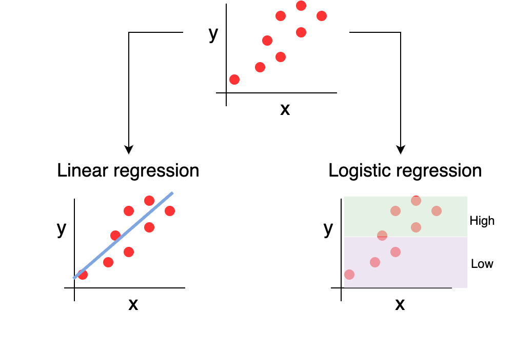
16.2.1 Linear regression
For linear regression, the response variable (or the dependent variable or the one on the y axis) is quantitative. The response variable is expressed as a linear combination of the predictor variables, i.e. \(\vec{y}=a_{0} + a_{1} x_{1} + a_{2} x_{2} + ... a_{n} x_{n}\), the so called “best-fit line”. Each term of the linear regression (\(a_{0}\), \(a_{1}\), etc) is directly proportional to the corresponding predictor variable (\(x_{1}\), \(x_{2}\), \(x_{3}\), etc). The parameters of the linear regression \(a_{i}\) all measure the rate of change in the response variable for a corresponding unit increase in the corresponding predictor variable. The regression coefficients are sometimes characterized as the effect of the predictor variable.
In mathematics when we say one variable is directly proportional to another variable (e.g. growth rate is directly proportional to temperature), the mathematical expression is growth rate = a\(\cdot\)temperature. We need the constant “a” here because it may not be a direct 1-1 relationship. Linear regression is used to help define that relationship. The key thing to note is that if the predictor variable increases by a factor (e.g. doubles) than the response variable will also increase by the same factor, no matter the value of the constant a. Let’s say we have \(y_{1} = a \cdot x_{1}\), and the value of \(x_{1}\) doubles, so \(x_{2} = 2 \cdot x_{1}\). Then \(y_{2} = a\cdot x_{2} = a\cdot (2 \cdot x_{1}) = 2 \cdot (a \cdot x_{1}) = 2 \cdot y_{1}\).
Linear regression can include a mixture of categorical predictor variables, or also effects of variables together (i.e. \(a_{ij} x_{i} \cdot x_{j}\), which \(x_{i} \cdot x_{j}\) could be considered a new variable \(y_{ij}=x_{i} \cdot x_{j}\)). Of note is to declare the variables as categorical or designate them as factor variables. If you have a mixture of categorical variables (i.e. not a simple binary), there may be some nuances and choices in coding these, which may also influence regression values.
Linear regression (and variants of it) are common in all computational software programs. Python uses the scikit-learn library, which also implements several other machine learning methods. Linear regression in R uses the function lm, which stands for linear models. The methods to compute linear regression also include statistical information (such as uncertainty estimates, significance, etc). Of note is the broom package for R for extracting these out in a data table friendly format.
16.2.2 Logistic regression
Moving from simple linear regression, logistic regression is used when the predictor variable is a binary response variable (such as indicating presence or absence of a species).
Logistic regression forms the basis of many classification algorithms in machine learning (Boehmke and Greenwell 2019; Carter 2020). Logistic regression predicts the probability (called \(\pi\)) of the predictor variable occurring, using the probability of 0.5 as a cutoff, as determined by the odds. The odds is defined as the ratio of the probability of success (\(\pi\)) of the variable occurring to failure (\(1-\pi\)), or expressed as \(\frac{\pi}{1-\pi}\). Because the odds has a domain of all positive numbers, in practice the log-odds is computed (\(\ln \left(\frac{\pi}{1-\pi} \right)\)), giving a range of all real numbers.
Logistic regression then models the log odds as a linear function, with the log odds being a response variable and (i.e. \(=a_{0} + a_{1} x_{1} + a_{2} x_{2} + ... a_{n} x_{n}\) as with linear regression). Algebraic manipulation then be transformed back into an equation that models the probability \(\pi\) as a logistic equation.. In R the engine that does logistic regression is glm, or in Python as LogisticRegression.
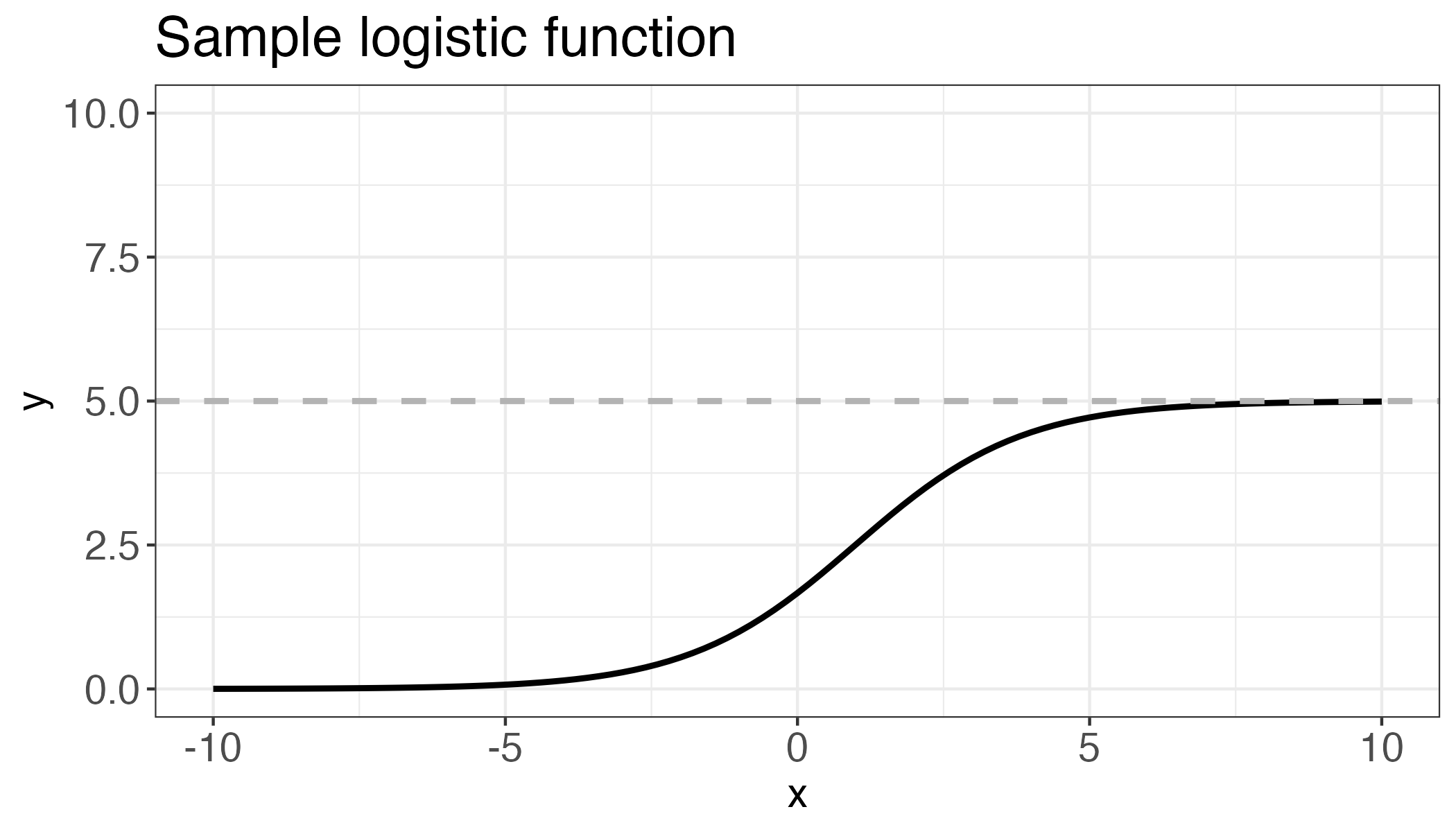
A logistic equation is sometimes described as an S-curve, due to its shape. Logistic equations are often used to describe limiting values, as opposed to linear or exponential growth which increases without bound. The expression for a logistic equation is \[\displaystyle y = \frac{K}{1+B \cdot e^{-rx}}\], where the parameter \(K\) refers to the carrying capacity or limiting value, \(r\) is the growth rate, and \(B\) is a constant related to the y intercept, or where the graph crosses the vertical axis. For logistic regression, \(K = 1\).
16.3 Process modeling
Another approach is dynamic modeling (Zobitz 2023). A fundamental building block for dynamic modeling is identifying (1) state variables and (2) processes that transform different state variables from one to another. One area where this could be examined is process-based ecosystem modeling. To provide a specific example, let’s focus on soil carbon and transformation. Figure 16.3 displays a conceptual diagram for a soil model, where state variables are represented with rectangular boxes and processes with arrows.
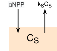
In this model we have a single pool, \(C_{S}\), that represents the amount of carbon in the soil (usually measured in grams carbon per square meter, or g C m-2). One process that carbon accumulates in the soil is through net primary production \(NPP\), or excess carbon generated from photosynthesis after respiration from aboveground components (leaves, stems, etc). In this case a proportion of \(NPP\) enters the soil from root exudates, which we can represent mathematically as \(\alpha \; NPP\), where \(\alpha\) is a proportionality constant. In the soil, microbes utilize carbon and then respire carbon as carbon dioxide. One way to mathematically represent the transformation by soil microbes is \(k_{S} C_{S}\), where \(k_{S}\) is a rate constant.
The dynamic model then describes the rate of change of soil carbon, \(\displaystyle \frac{dC_{S}}{dt}\) with the following equation: \[\displaystyle \frac{dC_{S}}{dt} = \alpha \, NPP - k_{S}C_{S}.\]
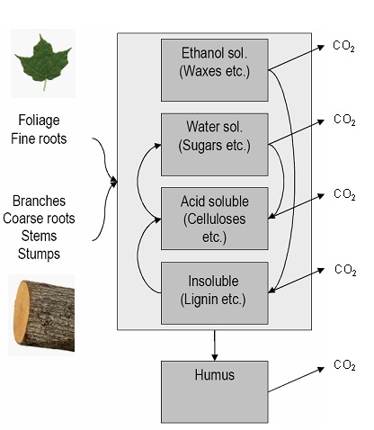
Figure 16.3 is a heuristic model that is most likely not suitable for prediction. Other refinements may include more state variables and processes for specific soil components. As an example, Figure 16.4 shows a conceptual diagram for the Yasso model (Liski et al. 2003; Liski et al. 2005). This model has many more state variables than our heuristic model above, notably specifying different types of soil compounds (e.g. sugars, ethanol, lignin), as that affects microbial decomposition.
One challenge with more complex models is parameterization. Utilization of model parameterization methods (Markov Chain Monte Carlo parameter estimation or other machine learning methods), as described next.
16.4 Bayesian modeling and machine learning
Another approach is Bayesian modeling. This approach is one that assumes that either the response variables, predictor variables, or regression parameters follow some probability distribution. This information about the distribution of variables or parameters is then incorporated into the statistical modeling, which may sharpen or define the resulting approaches. that you can incoporate that information into your workflow. For example, applying Bayeisan modeling to our heuristic model in Figure 16.3 to estimate the unknown parameters \(\alpha\) and \(k_{S}\) might assume distributions on each of the respective parameters. A dataset of soil respiration or measured soil carbon over time at a site could used to derive a data-informed estimate of the parameters \(\alpha\) and \(k_{S}\). Viskari et al. (2022) used such an approach to calibrate the Yasso model from a worldwide database of litter decomposition and soil organic carbon measurements.
Saying that a value follows a probability distribution means that you are indicating a state of belief (or sometimes known as probabilities) about its value. Probabilities range from 0 to 1. A probability distribution may refer to one of two concepts: the probability density function, which specifies the value for a state of belief about a value, or the cumulative distribution function, which represents the accumulated probability across the range of possible values for a variable.
Bayesian modeling is implemented through the MCMC (Markov Chain Monte Carlo) approach, which is a sequential algorithm that randomly explore the parameter space, evaluating whether to accept or reject a function based on the likelihood function (Zobitz et al. 2011). There are many considerations when doing Bayesian parameter estimation (Clark 2007; Gelman et al. 2014; Dietze 2017) which can be computationally intensive.
We mentioned machine learning in this subsection title as Bayesian parameter analysis is essentially a type of machine learning: both use algorithms to determine an optimal set of parameters given a specific target set. Machine learning is broadly categorized into supervised algorithms, which use a defined function to associate datasets (e.g., linear regression), and unsupervised algorithms, which identify patterns or structures within data without prior labels. While a deeper dive into these evolving techniques is beyond our current scope, Boehmke and Greenwell (2019), Kuhn and Silge (2022), and Géron (2023) are excellent resources for further study.
16.5 Causal inference
An emerging topic in environmental sciences is causal inference or causation (Cunningham 2021; Byrnes and Dee 2025). Much of statistics concerns itself with association - i.e. increased temperature is associated with soil respiration. Causal inference is the study of attribution - in other words soil respiration increases as a result of increased temperatures.
Isn’t this just semantics? Not really. Causation between two variables X and Y can defined in 4 different ways (X causes Y; Y causes X, X causes Y and Y causes X, or no causality). The number of ways that causation between two variables can be determined equals \(4^{N\choose 2}\) for \(N\) variables. If you have a dataset of several variables, you need to test all these different associations.
There are several approaches in which to determine causation:
- Granger causality (Granger 1969): relies on statistical associations between two timeseries variables (say \(x\) and \(y\). Briefly linear regression of \(y\) against lagged values of \(y\) are conducted. Then a second regression of \(y\) with lagged values of \(y\) and lagged values of \(x\) are conducted Causality is determined in a statistical sense to see if including lagged values of \(x\) increases explanatory power of \(y\)
- Transfer entropy (Schreiber 2000): borrows concepts from information theory to measure the Kullback-Leibler divergence. In this case, the Kullback-Leilbler divergence compares distribution of \(y\) and \(x\) (both with lags) to the distribution of \(y\) by itself. Significance is often estimated through bootstrapping, which may slow down processing time.
- Convergent cross mapping applies a dynamical systems approach to determine causality. It views two separate timeseries as a projection of a complex dimensional space called a manifold. The goal is to reconstruct the manifold using the lagged timeseries. A good video primer on this elegant theory is found here: LINK
While briefly outlined here, causal inference is quickly becoming a necessary tool (along with advances in machine learning) for processing large datasets that may be associated with each other (Ferraro et al. 2019; Ombadi et al. 2020; Siegel and Dee 2025).
16.6 Exercises
- Chapter 2 introduced datasets of reported weather and streamflow data (Figure 2.4) for the Mississippi in St. Paul, Minnesota. Figure 16.5 displays the reported values in 2024 of maximum temperature (
max_temp), minimum temperature (min_temp), and precipitation (precip) at each day. Use this information to answer the following questions:
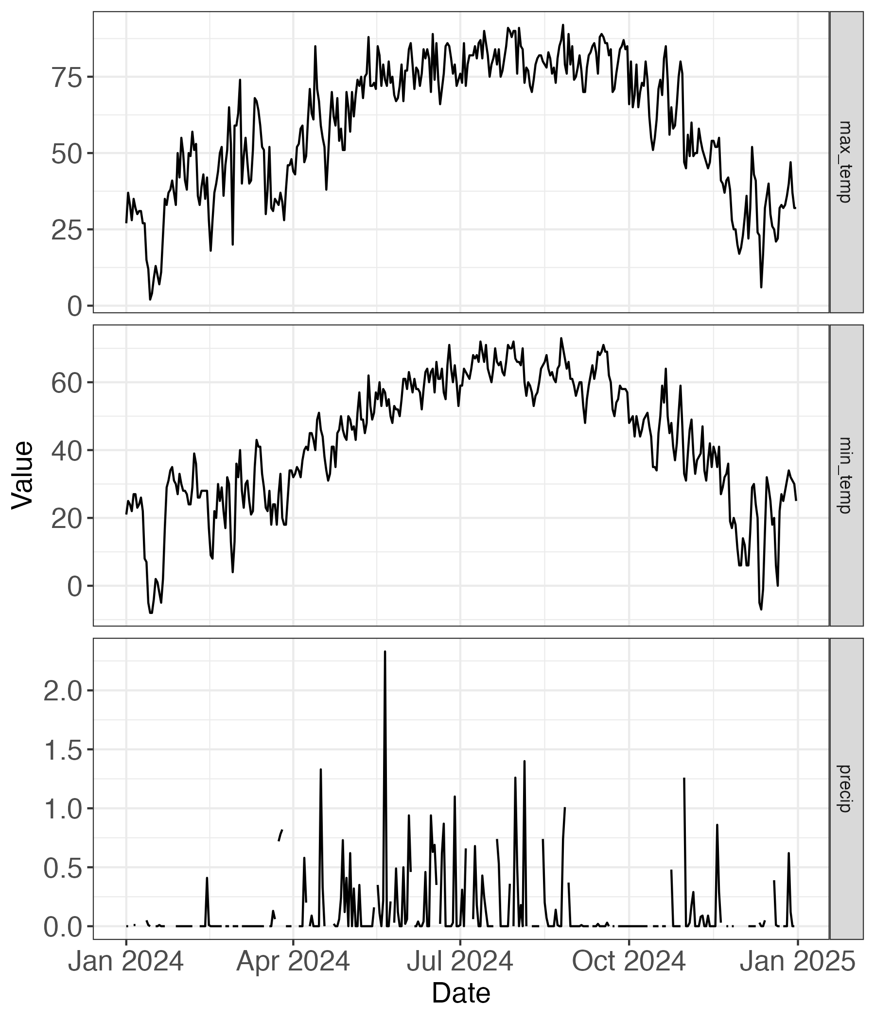
max_temp is the maximum temperature (degrees Fahrenheit), min_temp the minimum tempreature (degrees Fahrenheit), and precip daily precipitation (inches).
a. What would be a causal diagram that might influence how the variables presented in the graph relate to each other?

b. What would be a possible scenario where you were to apply linear regression to these variables?

c. What would be a possible scenario where you were to apply logistic regression to these variables?- For logistic regression, the binary response variable is based on the probability \(P\) of the event happening, with \(P=0.5\) being the cutoff for success and failure of the binary response variable. The odds of the variable is defined as \(\displaystyle \frac{P}{1-P}\), and the log-odds as \(\displaystyle \ln \left( \frac{P}{1-P} \right)\). If \(P=0.5\), what are the values of the odds and log-odds? If \(P<0.5\)? \(P>0.5\)?