13 Wrangling and joining data

As a data scientists, one of the fundamental tasks is data transformation starting with flat files or a spreadsheet. The goal of transformation is to extend analyses beyond just the observations. How you transform the data depends on the scientific questions you are exploring - and can include summary statistics or applying a mathematical model. This process is called data wrangling and places the emphasis on action - what do you want to do with your data today?

Similarly, spreadsheet programs (e.g. Google Sheets, Microsoft Excel, or Apple Numbers), do have limitations on the amount of data to be utilized. Data volume is a consideration when doing data transformation with spreadsheets. Microsoft Excel is limited to about a million observations and 16 thousand variables - which may seem like a lot, but processing with a spreadsheet program can easily get swamped when the number of observations increase. As an alternative, data can be stored in smaller files that are linked together, which is called a join. This chapter is focused on data wrangling and connecting two data tables together. Let’s begin.

13.1 What’s the weather like?

Minnesota loves to talk about its weather, reflected in a strong tradition of long-term, high-quality weather observations.¹

Weather data for Minnesota and other states are easily accessible through the Iowa Environmental Mesonet. We accessed the data from 2023 from the MSP station, which provided over 10000 observations of air temperature (labeled tmpf), dewpoint (labeled dwpf), and relative humidity (labeled relh). We will call this dataset msp_2023. A sample of this dataset is shown below:

Rows: 365
Columns: 6
$ day            <date> 2023-01-01, 2023-01-02, 2023-01-03, 2023-01-04, 2023-0…
$ max_temp_f     <dbl> 35, 27, 31, 33, 30, 19, 21, 25, 32, 28, 34, 32, 20, 31,…
$ min_temp_f     <dbl> 22, 22, 24, 30, 18, 5, 0, 0, 8, 19, 26, 19, 13, 13, 29,…
$ max_dewpoint_f <dbl> 28.0, 21.9, 28.9, 30.9, 27.0, 14.0, 10.9, 15.1, 27.0, 2…
$ min_dewpoint_f <dbl> 18.0, 19.4, 19.9, 27.0, 15.1, 1.0, -5.1, 0.0, 6.1, 17.1…
$ avg_rh         <dbl> 83.36661, 87.41795, 87.52398, 91.89084, 83.86404, 82.04…

In the following sections we will use this dataset to introduce two fundamental data wrangling actions: transforming and summarizing data.

13.1.1 Creating new variables

The documentation for dataset msp_2023 reports that the air temperature and dewpoint variables (max_temp_f ,min_temp_f ,max_dewpoint_f,min_dewpoint_f) are provided in degrees Fahrenheit, which is the standard way to report temperature in the United States.² Typically environmental science analyses use the SI (Metric) system where temperature is reported in degrees Celsius. Do you recall the formula for conversion between Fahrenheit and Celsius? The formula is $\displaystyle T_{C} = \frac{5}{9} \cdot(T_{F}-32)$ where $T_{C}$ is the temperature in Celsius and $T_{F}$ the temperature in Fahrenheit.

Creating a new variable from existing observations is an example of a data mutation or transformation. In this instance you are not changing the number of rows in a data table but rather adding a new variable, according to a formula. Sample code in the R syntax with a variety of different approaches is shown below:

msp_2023_new <- mutate(msp_2023,
  max_temp_c = 5 / 9 * (max_temp_f - 32),
  min_temp_c = 5 / 9 * (min_temp_f - 32),  
)

# Alternative for using pipes:
msp_2023_new <- msp_2023 |>
  mutate(
    max_temp_c = 5 / 9 * (max_temp_f - 32),
    min_temp_c = 5 / 9 * (min_temp_f - 32), 
  )

# Base R
msp_2023_new$max_temp_c <- 5 / 9 * (msp_2023$max_temp_f - 32)
msp_2023_new$min_temp_c <- 5 / 9 * (msp_2023$min_temp_f - 32)

Spreadsheet programs could also accomplish the same tasks, but coding these steps into a script file (whether in Python, R, or Julia) allow for the workflow to be easily adapted if new data are incorporated, which is sometimes termed data wrangling.

13.1.2 Rolling up a dataset

Another fundamental data wrangling task is summarizing data based on the input. Given the dataset of daily weather observations, some good questions we could ask of these data are:

How many of observations per day are there?
What is the average daily high for the entire year?
What is the average daily low for the entire year?
What is the average monthly temperature?

These questions represent a gamut of data wrangling tasks that involve summarizing or “rolling up” a dataset. To compute the average high temperature in Minneapolis/St. Paul in 2023 we will need to take the entire vector of maximum temperature (max_temp_f) and computing a mean value from the observations, which works out to be 58.6 $^{\circ}$F. The process of rolling up the maximum temperature is schematically shown in Figure 13.1:

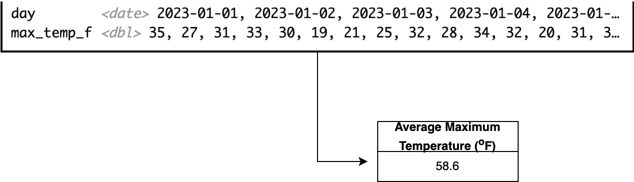
Schematic diagram illustrating the concept of rolling up a data set. This is represented with a flow diagram of two vectors day and max_temp_f flowing into a single output of average maximum temperature. — Figure 13.1: Schematic of summarizing the maximum daily temperature in Minneapolis/St. Paul observations to compute the average maximum temperature as a single value.

The key distinction between mutating (adding new variables) and summarizing data is that summarizing produces a single observation from a set of vectors, whereas a mutating retains the same number of observations as the input.

Another use-case for summarizing is computing a value across different groups, such as when you have a categorical variable. For our dataset of weather observations, to compute the average maximum monthly temperature, we would first need to separate the msp_2023 dataset into observations for each month, and then compute the average in each month. Typically when we summarize a dataset we often want to look at results from cases for a categorical variable. This process is called grouping and summarizing.

Figure 13.2 illustrates a schematic diagram of grouping and summarizing for the Minneapolis/St. Paul temperature data. Behind the scenes what the code first subsets the data into each instance of the categorical variable specified (in this case, the month), and then computes the average temperature across each subset. The result is a data frame with two variables: month and average temperature.

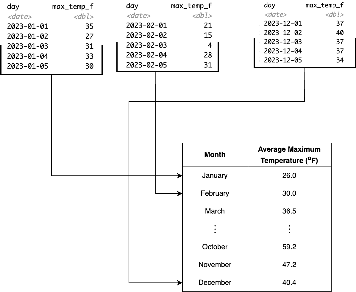
Schematic flowchart that illustrates a grouping and summarizing. Data of day and max_temp are separated into each month at the top of a diagram. Each month then has arrows leading to a summary table with columns month and average maximum temperature in degrees Fahrenheit. — Figure 13.2: Schematic of summarizing the maximum daily temperature observations for each month in 2023 for the `msp_2023` dataset, illustrating a grouping and summarizing action.

The following Python code below will determine the specific month from our data frame and then group by the month to compute the average temperature:

import pandas

msp_2023['month'] = msp_2023['valid'].dt.month  # Extract month

monthly_avg = msp_2023.groupby('month')['max_temp_f'].mean(skipna=True)

13.2 Vectors on my mind

A transformative aspect to the concept of data wrangling is the notion of considering data as vectors, in other words a collection of information versus a single observation. Having a dataset that is considered “tidy” is a good first step towards vectorization (Wickham and Grolemund 2017). The msp_2023 data table could be considered a tidy dataset - each row is an observation (different day of the year), and each column represents a variable.

When we converted the temperature data from Fahrenheit to Celsius, we applied a single formula to each of the different observations. Schematically, Figure 13.3 demonstrates this action with each of the blue dashed arrows starting from the variable max_temp_f to the new variable max_temp_c. More abstractly, a vectorized operation applies the same formula (expressed in the blue box as C = 5/9*(F-32) in Figure 13.3).

Schematic diagram illustrating vectorized operations. There are three columns in the figure, the first one is day, indicating sequential year month day of 2023. The second column is the corresponding temperature in degrees Fahrenheit. A blue arrow extends from each Fahrenheit temperature to the third column, which is the maximum temperature in degrees Celsius. Above the first arrow is a blue box that converts Fahrenheit temperatures to Celsius using the named variables. The bottom of the figure has three orange boxes underneath each column with text of day, F, and C respectively. There is also a blue box representing the conversion formula from Fahrenheit to Celsius. — Figure 13.3: Converting temperature data from Fahrenheit to Celsius, through applying the same formula one at a time across all temperature observations to create a new variable. Considering each variable as a vector (orange boxes at the bottom) illustrates the vectorized workflow.

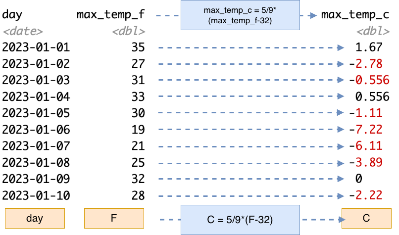
For a small dataset the one-at-a-time approach in Figure 13.3 works well. If you were to apply this conversion in a spreadsheet program, you would perhaps create a new column with a formula and references to the cell in the previous column over, and then “fill-in” the remaining entries, which applies the same consistent formula across everything.

For small to medium-sized datasets spreadsheet programs are very efficient. However for the msp_2023 dataset, we most definitely would not want to apply that same formula 365 times! Rather, imagine the collection of maximum Fahrenheit temperature observations together (represented by the orange box F in Figure 13.3). In this case we are applying a single formula to produce the vector C in Figure 13.3 (orange box C in Figure 13.3). While this may seem like sleight of hand, vectorized thinking helps to simplify your thinking when doing analyses. In this way we can consider a single action to a variable (which consists of a set of observations) instead of actions on each individual operation. The alternative if we didn’t have this efficiency of scale is to write iterative loops, which do consume computational time (Chapter 14). Iterative loops have their purpose, but not as a substitute for vectorized code.

13.3 Joins

This whole time we have been focused on a single data table but in many cases all the information that you need for a project isn’t contained in a single data table - and this is the power of data science is the combination of different data tables together.

Joins are also a helpful data management tool because it allows you reduce that cognitive load that may come with a dataset with a large number of variables. Another bonus is that the computer’s cognitive load (i.e. memory) is easier when working with smaller datasets - importing several smaller datasets requires less in-memory usage than a single large dataset.

As an example, we also examined the daily temperature data in Lawrence, Kansas where Naupaka is located. We will call this data table lwc_2023. This data table has the same structure as msp_2023:

Rows: 365
Columns: 6
$ day            <date> 2023-01-01, 2023-01-02, 2023-01-03, 2023-01-04, 2023-0…
$ max_temp_f     <dbl> 61, 54, 52, 48, 48, 51, 40, 51, 60, 58, 54, 37, 33, 49,…
$ min_temp_f     <dbl> 26, 41, 34, 30, 21, 16, 26, 17, 23, 22, 24, 27, 16, 16,…
$ max_dewpoint_f <dbl> 43.0, 52.0, 51.1, 26.1, 24.1, 27.0, 25.0, 27.0, 34.0, 3…
$ min_dewpoint_f <dbl> 25.0, 36.0, 24.1, 19.0, 17.1, 14.0, 17.1, 14.0, 19.9, 2…
$ avg_rh         <dbl> 75.74717, 90.79071, 75.91724, 56.44588, 64.28067, 64.68…

Our two datasets msp_2023 and lwc_2023 measure the same variables. One possible action it to combine the datasets together for ease of comparison. The fundamental way to join variables together is to the presence of a key - which is the same variable from two different data tables. The key to join these two data tables together is the variable day. Sometimes keys are easy to identify (the variable may be named the same across data tables). In cases where it is not, you will need to consult the provided data dictionaries to identify the corresponding names.

The most common type of join is the intersection or what we call the inner join. When we join these msp_2023 and lwc_2023 together in R with an inner join we obtain the resulting data table:

Rows: 365
Columns: 11
$ day              <date> 2023-01-01, 2023-01-02, 2023-01-03, 2023-01-04, 2023…
$ max_temp_f.x     <dbl> 35, 27, 31, 33, 30, 19, 21, 25, 32, 28, 34, 32, 20, 3…
$ min_temp_f.x     <dbl> 22, 22, 24, 30, 18, 5, 0, 0, 8, 19, 26, 19, 13, 13, 2…
$ max_dewpoint_f.x <dbl> 28.0, 21.9, 28.9, 30.9, 27.0, 14.0, 10.9, 15.1, 27.0,…
$ min_dewpoint_f.x <dbl> 18.0, 19.4, 19.9, 27.0, 15.1, 1.0, -5.1, 0.0, 6.1, 17…
$ avg_rh.x         <dbl> 83.36661, 87.41795, 87.52398, 91.89084, 83.86404, 82.…
$ max_temp_f.y     <dbl> 61, 54, 52, 48, 48, 51, 40, 51, 60, 58, 54, 37, 33, 4…
$ min_temp_f.y     <dbl> 26, 41, 34, 30, 21, 16, 26, 17, 23, 22, 24, 27, 16, 1…
$ max_dewpoint_f.y <dbl> 43.0, 52.0, 51.1, 26.1, 24.1, 27.0, 25.0, 27.0, 34.0,…
$ min_dewpoint_f.y <dbl> 25.0, 36.0, 24.1, 19.0, 17.1, 14.0, 17.1, 14.0, 19.9,…
$ avg_rh.y         <dbl> 75.74717, 90.79071, 75.91724, 56.44588, 64.28067, 64.…

In our example msp_2023 and lwc_2023 have other variables that are named the same beyond the key of day (i.e. max_temp_f ,min_temp_f ,max_dewpoint_f,min_dewpoint_f) . That can be an issue when joining two data tables. In this case, the join function appends a .x and .y to each variable signify if they are from the first (.x) or second dataset (.y). Depending on the context these variables could be renamed.

Once the tables are joined, it might be interesting to see how the two locations vary in temperature or dewpoint. We will leave that up to work out as an exercise in Section 13.5.

Your intuition is on the right track if an inner join reminds you of the overlapping section of a Venn diagram. In fact, many join operations correspond to familiar set relationships. For example, left joins and semi joins (among others) each capture different ways of combining data from two tables.

One additional consideration is what happens when a table contains repeated values in the key column. These duplicate keys can lead to multiple matches, which can change the size and structure of the resulting dataset. Understanding how different joins behave—and how they handle duplicate keys—is essential for working effectively with real-world data.

13.4 Code switching

Programming languages such as R, Python, and Julia all have functions that manage wrangling and joining datasets (such as Wickham and Grolemund (2017), Baumer et al. (2021), or McKinney (2022)). The challenge is that the names of the functions for data wrangling and joining and how they are implemented may vary. Table 13.1 showcases different examples of data wrangling and joining functions across R and python:

Table 13.1: Comparison of different data actions and the key functions used in Python, R, and Julia.

Action	Base R	tidyverse (R)	pandas (Python)
Create new variables	`x$var_x <- FORMULA`	`mutate`	`transform`
Extract variables	`x[,'name']`	`select`	`x[['col1']]`
Arrange variables	`order`	`arrange`
Change variable name		`rename`
Change variable order in data table		`relocate`
Roll up data	`by` with `do.call`	`summarize`	`aggregate` or `agg`
Grouping	`aggregate`	`group_by`	`.groupby`
Inner join	`merge`	`inner_join`	`merge`

13.5 Exercises

Datasets msp_2023 and lwc_2023 as csv files can be found in the eds-text-data github repository

For the msp_2023 and lwc_2023 datasets separately, calculate the average minimum temperature for each month.
For the msp_2023 and lwc_2023 datasets separately, calculate the root mean square error (RMSE) of the maximum and minimum temperature for each month. Are there any seasonal trends that you notice?
Compute the median of the maximum and minimum temperature each month for the msp_2023 and lwc_2023 datasets separately. Join the two datasets together. You might need to rename columns, but make a visualization comparing the two locations and their temperatures over the course of the year.
A simple rule of thumb is that dewpoint, or the temperature that water vapor is cooled to saturation decreases by one degree Celsius for every 5% decrease in relative humidity (Lawrence 2005). Mathematically, the formula would be $\displaystyle T_{d} = T_{C} - \frac{100-RH}{5}$, where $RH$ is the relative humidity and $T_{C}$ is the temperature in Celsisus.
1. Use the formula $\displaystyle T_{C} = \frac{5}{9} \cdot(T_{F}-32)$ to express this rule of thumb formula as a function of $T_{F}$ and $RH$.
2. Using the expression you just developed and the msp_2023 dataset, create a new variable called max_dewpoint_f_5 (relative dewpoint with the 5% rule of thumb) using the maximum temperature.
3. Repeat the same process with the minimum temperature. Call this variable min_dewpoint_f_5.
4. Generate a scatter plot comparing max_dewpoint_f_5 to max_dewpoint_f and min_dewpoint_f_5 to min_dewpoint_f.
5. Dewpoints are a function of vapor pressure and temperature and are typically measured through a scientific sensor (as reported in the documentation). Compare the rule of thumb to the measured variable dwpf. How does the rule of thumb compare in a 1-1 plot?
6. Compute the root mean square error in the dataset of for each month. Are there any seasonal trends that you notice?

As an example, the state maintains high-quality datasets of weather observations from backyard observers.↩︎
The names of the variables have _f, also suggests this context if you don’t have the data documentation at hand.↩︎