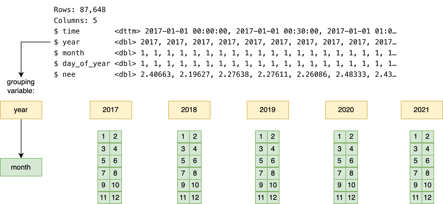
Rows: 87,648
Columns: 5
$ time        <dttm> 2017-01-01 00:00:00, 2017-01-01 00:30:00, 2017-01-01 01:0…
$ year        <dbl> 2017, 2017, 2017, 2017, 2017, 2017, 2017, 2017, 2017, 2017…
$ month       <dbl> 1, 1, 1, 1, 1, 1, 1, 1, 1, 1, 1, 1, 1, 1, 1, 1, 1, 1, 1, 1…
$ day_of_year <dbl> 1, 1, 1, 1, 1, 1, 1, 1, 1, 1, 1, 1, 1, 1, 1, 1, 1, 1, 1, 1…
$ nee <dbl> 2.40663, 2.19627, 2.27638, 2.27611, 2.26086, 2.48333, 2.43…14 Iteration without tears
What is the best way to begin a complex project? Answers undoubtedly may vary, but a common approach is to break the project down into smaller, manageable steps to complete. We tend to approach data science projects in a similar way, assembling the pieces into a large whole along the way. This type of project management workflow is an example of the computing concept of split-apply-combine (Wickham 2011); Chapter 5 also used this approach in project management.
Many computational aspects for environmental data science require you to apply the same process or procedure across a set of groups. Perhaps you are computing annual biomass accumulation across a set of different sites, or testing the statistical significance of a treatment effect in a factorial experiment. For these computations you will need to apply the concept of iteration, which is part of workhorse to make split-apply-combine work so well. Benefits of iteration are to (1) reduce computational time, (2) improve code readability, or (3) emphasize process. In this chapter we examine a case study where iteration is used for aggregation. Let’s begin.
14.1 Case study
Data collected through the eddy covariance technique represents the net amount of carbon exchanged between an ecosystem and the atmosphere in a defined footprint area; this measurement is called Net Ecosystem Exchange of Carbon, or NEE for short. NEE is a key output for terrestrial carbon models as well as important to scaling up carbon exchange from local to regional scales (Baldocchi 2014).
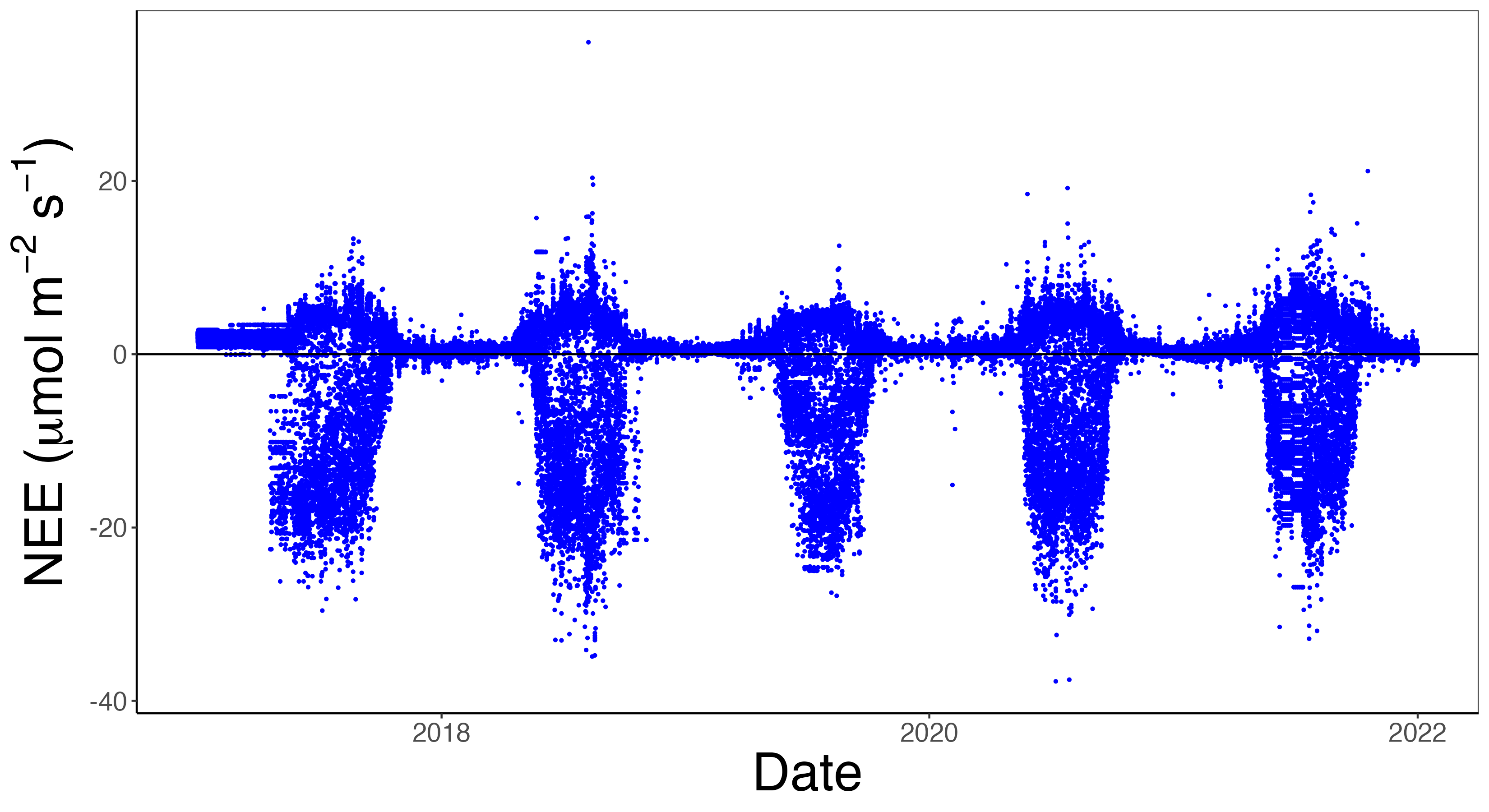
FLUXNET is a consortium of networks across the globe that provide access to NEE and other associated measurements. Because the base measurement of NEE is averaged over a half hour, and typically NEE is reported in units of \(\mu\)mol CO\(_{2}\) m\(^{-2}\) s\(^{-1}\). As an example of NEE, we’ve identified data from the University of Notre Dame Environmental Research Center. A sample of the dataset is shown below:
The dataset above can be plotted as a timeseries, shown in Figure 14.1, with the variable NEE on the vertical axis and day_of_year on the horizontal axis. Notice that NEE is measured in \(\mu\)mol CO\(_{2}\) m\(^{-2}\) s\(^{-1}\), which through a unit conversion can be computed to gC m\(^{-2}\) half-hour\(^{-1}\). The multiyear dataset allows us to see distinct seasonal patterns due to springtime and summer in the northern hemisphere. In Figure 14.1 we utilize the convention that negative values of NEE indicate the ecosystem is a net carbon sink; positive values means the ecosystem is a net carbon source to the atmosphere.
14.2 Iteration approaches
Let’s now focus on a task that requires variations on iteration. A common task when working with half-hourly NEE data (as shown in Figure 14.1) is compute monthly NEE values, reported as gC m\(^{-2}\) month\(^{-1}\). In order to accomplish this requires completing several intermediate steps:
- identifying all measurements in a given month, for a given year
- converting to \(\mu\)mol CO\(_{2}\) m\(^{-2}\) s\(^{-1}\) to gC m\(^{-2}\) half-hour\(^{-1}\). We will use the conversion that 0.0216198 gC m\(^{-2}\) half-hour\(^{-1}\) = 1 \(\mu\)mol CO\(_{2}\) m\(^{-2}\) s\(^{-1}\).
- aggregating these values each month, using the Fundamental Theorem of Calculus (Zobitz 2013)
This computation will require some iteration. We will present some approaches to computing monthly totals using the R language and dplyr package. Although we are focused on R, they can easily be adapted to Python or Julia.
14.2.1 Iteration with for loops
The for and variants (e.g. while) are perhaps the go-to iteration method. For most programming languages the for loop requires pre-allocation of an output vector (if that is what is needed), with the for loop “filling up” the entries of the output vector as you go.
In our example, computing monthly NEE with a for loop requires:
- Determining the number of unique years and months
- Allocation of the data frame to store the monthly values.
- Looping through each year and month, subsetting the NEE data, converting, and computing the total.
- Appending the sum and the current month and year.
Here is some example R code to accomplish compute monthly NEE:
# Determine the years and months
unique_years <- unique(unde_nee$year)
unique_months <- unique(unde_nee$month)


# Create an empty data frame to store results
nee_monthly <- data.frame(
  year = integer(),
  month = integer(),
  tot = numeric()
  )


# Loop through each year and month combination
for (y in unique_years) {
  for (m in unique_months) {
    # Subset data for the given year and month
    subset_data <- unde_nee[unde_nee$year == y & unde_nee$month == m, ]

    # Compute the total NEE for the given month
    total_nee <- sum(subset_data$nee * 0.0216198, na.rm = TRUE)

    # Append to results
    nee_monthly <- rbind(nee_monthly,
                         data.frame(year = y, month = m, tot = total_nee)
                         )
  }
}
Because we have a multi-year dataset, we needed a nested for loop (one for year and another for each month of that year). In Section 14.4 you will try to write a single for loop.
14.2.2 Iteration by grouping and summarizing
Summarizing in data science refers to the process of taking a vector of information and producing a single output (Wickham and Grolemund 2017; Baumer et al. 2021). Examples of a summary function include the computing the mean (average) of data, standard deviation, or other summary statistics. Summarizing is also known as “rolling up” a dataset.
A related concept to summarizing is grouping, which sorts a multifactor dataset by a categorical variable. For the unde_nee data, we could group our data by the variables year and month, as we wish to compute the total NEE value in each distinct year and month. Typically grouping is used in conjunction with summarizing as an alternative to iteration.
Arguably grouping and summarizing is iteration by systematically subsetting the data by a categorical variable and applying the same function to each subset, producing a single result. The dplyr package for R provides versatile functionality to compute the monthly values - we can use the sum function to the variable nee after applying our unit conversion:
unde_nee |>
  group_by(year,month) |>
  summarize(tot = sum(nee*0.0216198))
In the code above, first what happens is the data are split up into separate years, and then for each year, split up into each month. Figure 14.2 illustrates a conceptual diagram of the grouping and summarizing process.
When using group_by in R, information about the original data is retained in the grouping structure as metadata; for larger datasets this original information may slow down processing and consume in-computer memory.1
Now that we have grouped and summarized the data, Figure 14.3 shows a timeseries of each year stacked on top of each other. This timeseries allows for the comparison across years. We utilized a similar approach in Chapter 1 when we were investigating soil temperature across multiple years.

14.2.3 Iteration using map functionals
A third approach to iteration uses the concept of functionals (e.g. functions), represented in the purrr package as map and its variants. These functionals are examples of the most general (and versatile) example of map-reduce (Dean and Ghemawat 2004) or split-apply-combine (Wickham 2011), where the dataset is divided into smaller chunks for processing.
The key to understanding map functionals are nested lists, which generalizes the idea of a data frame. We introduced lists in Chapter 2. A nested list still follows the convention of “tidy” data where each row is an observation and each column a variable. But in this case, an “observation” may be another data table.
A helpful metaphor of a nested list. is a backpack where the primary pocket contains my notebook, computer, and textbook, but the side pocket contains a collection of pens (red, blue, black), stylus, and highlighters (orange, yellow). The backpack is analgous to the data table, with two variables: learning materials (notebook, computer, textbook) and writing materials (pens, stylus, and highlighters) the list. Here the writing materials corresponding to each learning material differ in size (3, 1, and 2 respectively).
The basic idea behind map is to apply a function that takes a collection of inputs and produces and output. See Chapter 9 in Wickham (2019) for more information on how to apply these functions. Some code to do this is shown below:
unde_nee |>
  group_by(year,month) |>
  nest() |>
  mutate(tot = map_dbl(.x=data,.f=~(sum(.x$nee*0.0216198))))
Nested lists are useful in cases where you may want to retain datas groups for additional processing or organization. The downside is that large nested lists may consume computer memory; it is helpful to evaluate if computing a data table output is better.
14.2.4 Timing
While we have presented three different options to compute the monthly NEE values from half-hourly data, let’s compute which is faster. The results are shown in Table 14.1.
We can compare the overall time of each iteration approach in Table 14.1.
| Approach | Time (seconds) |
|---|---|
for loops |
0.067 |
group_by → summarize |
0.034 |
map |
0.069 |
We recognize that timing of code is a subjective measure, as each computer differs in processing speed. But this does give an indication of the amount of resources needed.
Examining Table 14.1 shows that the group_by → summarize approach is by far the fastest. The dplyr (and also the data.table packages) are optimized for computing across groups. A quick internet search for optimizing dplyr shows that this is an active area of discussion, especially compared to the data.table package. If an iterative loop runs slow it is pause to think through assumptions and re-examine any approaches for efficiency.
14.3 Why iteration?
Now that we have seen some use cases of iteration, let’s take a step back and understand reasons for mastering iteration. The primary reason is efficiency: no one wants to rewrite code again and again, or worse, copy and paste the same code over and over making a small tweak. Speaking from experience, repasting code may introduce some unnecessary errors that are time consuming to fix.
A good rule of thumb when it becomes necessary to iterate:
TipIteration rule of thumb
do once → do twice → do many times
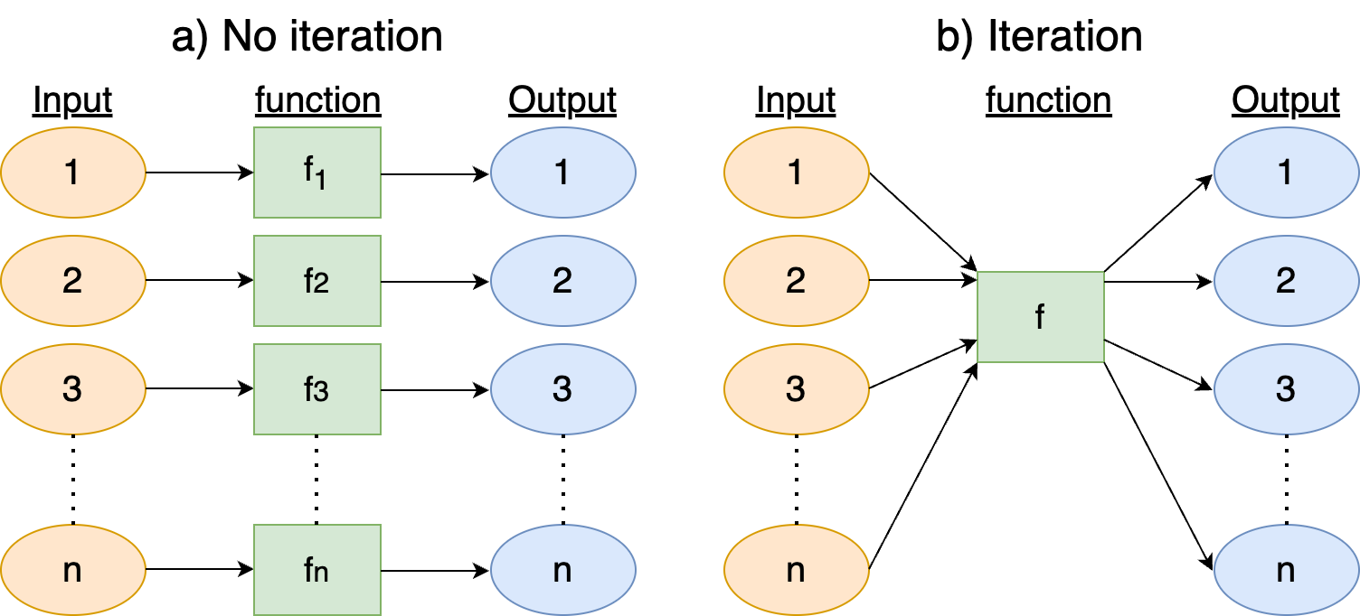
The goal of iteration is to focus your code and to focus on the product. Without iteration (left panel of Figure 14.4) you are making n different variations of the function f, which may mean copying and pasting (inefficient!), also opening up to a mistake. With iteration (right panel of Figure 14.4), you can focus on the optimizing the function f itself, and now that the identical process is applied to all groups.
Iteration works really well on vectorized operations - meaning that vectors, data frames, lists, and other data structures. R, Python, and Julia are well optimized to work with vectorized operations. One challenge for iteration is memory allocation - depending on the coding language pre-allocation of the output vector should be declared first. In R, sometimes outputs can be allocated on the fly. Syntax is important to consider. R requires the use of curly braces ({}), python requires indentation for the loop body, and julia the function end to close off the loop. Admittedly these are annoying to keep straight in your head - but not insurmountable. Each programming language has its own syntactical quirks when coding iterative loops.
Willingness to consider iteration also speaks to the iterative process of code review and refinement. Perhaps when you begin a project you get to an ending point. In reality, this ending point is the end of the beginning - there is still more ways to improve upon the first edit. Like drafts to papers you may revise, add comments, improve readability and flow, and perhaps think of an audience of the code beyond just ourselves. Mastering iteration is a powerful partner and tool to expand your analyses in efficient ways. Don’t be afraid to jump in and try iteration!
14.4 Exercises
Note: For these exercises, you can find the dataset unde_nee located here: LINK
Verify the unit conversion that 1 \(\mu\)mol CO\(_{2}\) m\(^{-2}\) s\(^{-1}\) = 0.0216198 gC m\(^{-2}\) half-hour\(^{-1}\).
The examples presented here use the
forloops in the R language for loops. Rewrite them in Python and Julia (or use AI to help you translate them.)In the NEE case study (Section 14.1), the
group_by→summarizeapproach usedyearandmonthhad the codegroup_by(year,month). What happens if you havegroup_by(month,year)? Explain why this is the case.In the NEE case study (Section 14.1), the
group_by→summarizeapproach usedyearandmonthas grouping variables. What happens to the result if you grouped only byyear? Only bymonth?The
data.tablepackages orapplyfunctions (base R) are also alternatives to computing the grouping and summarizing. Do the same computation as the NEE case study (Section 14.1) using these approaches.In the NEE case study (Section 14.1), the use of a nested
forloop can slow down code for large vectors, and sometimes swapping the order of the nests improves efficiency. Is there a difference in timing swapping the years and months loop?Rewrite the nested
forloop in the NEE case study (Section 14.1) as a single one. You may want to create a new data frame that contains all the different years and the months together.Use one of the iterative techniques described here and the
unde_needata to compute daily NEE values. In this case your output value will be NEE with units gC m\(^{-2}\) day\(^{-1}\).
If you want the resulting output to be a pure data table, you can use the option
.groups='drop'in thesummarizefunction, or also just use theungroup()function after the final result.↩︎