17 Data Science Workflows III: Workflow execution approaches and tools
This chapter will develop workflow execution tools, such as the process of writing and refining a makefile for a data science project. This is meant to be a culminating chapter synthesizing skills from the previous chapters.
17.1 Coding confessionals
We would be the first to admit that we are far from perfect with our project management. One key lesson of this book is that a growth mindsets (compared to fixed mindsets) are a healthy approach to programming. It is also instructive to hear “confessionals” of some of our practices that have worked well (or not so well).
17.1.1 John’s dirty song of ice and fire
In 2020 I received a Fulbrght scholar opportunity to collaborate with colleagues at the University of Eastern Finland in Kuopio, Finland. From previous field experiments my collaborators investigated changes in soil biogeochemistry across a fire chronosequence in Canada (Aaltonen, Köster, et al. 2019; Aaltonen, Palviainen, et al. 2019; Köster et al. 2017; Köster et al. 2024). Some of these data include soil carbon respiration, which showed varied responses across the century-long chronosequence. While the field work had all been completed, my task was to add more modeling aspects to understand processes affecting the soil decomposition and recovery at each site in the chronosequence (Zobitz et al. 2021).
The field data at hand was all contained within an spreadsheet - to which I also layered on additional data sources to corroborate the measurements.
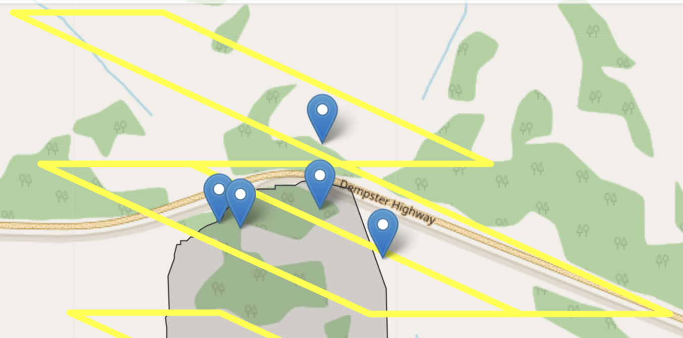
One the additional dataset was remote sensing data from NASA’s MODIS satellite, which is accessed via a web portal called A\(\rho \rho\)ears A\(\rho\rho\)ears (AppEEARS Team 2020). A satellite data product I was examining was gross primary producitivty (\(GPP\)). A \(GPP\) observation is calculated from derived measurements of photosynthetic fraction of absorbed radiation (Running and Zhao 2019). After preparing scripts to plot the timeseries of the data, the site that was most recently burned had no reduction in \(GPP\) - which is counterintuitive to a stand-replacing fire at this site. I needed a second source of corroborating evidence to understand this pattern.
To investigate this furthed I needed to access reported fire boundary data (Canada, n.d.) and compared it to the geographic boundaries seen by the MODIS pixel. After checking the two (Figure 17.1) it was appropriate to assume that the reported \(GPP\) came from an unburned forest. To proceed with the analysis we used a supplemental pixel entirely within the fire boundary as a proxy for \(GPP\).
To summarize, so far for this project I needed to do the following:
- Download data stored from a web service, which included text data and other geospatial data formats (Lovelace et al. 2019).
- Process and wrangle timeseries data then verify if they were consistent with observations.
- Visually compare geographic boundaries between two different areas.
Because I had several different data sources, the organization method included the following: - Two separate folders for data: raw-data (from websites above, other field observations) and data (derived data products I computed locally). - A folder for processing data (called data-process) This contained a series of script files that processed raw data into data for modeling. - A folder for general purpose R functions that could be used across all script files (a local library of functions) - A folder for analysis, containing script files that processed modeling data into outputs. - A folder for manuscript figure processing, which contained script files to generate manuscript figures. - A folder for the manuscript drafts and text.
While this seems like a logical approach, this was not my first attempt at project management. I had started with a single folder for data and script files. This quickly ballooned, and since all the files were quickly becoming interconnected, made it hard to see next action steps of how the different pieces related together.
For each of the script folders (for processing) the files were numbered in order of analysis, just in case when I needed to re-run analyses than I could do them in the correct order (at that time I was inexperienced with makefiles, but that would have been a huge help here!).
This organizational structure helped me keep the data science workflow into a few separate aspects (data acquisition, data analysis, modeling, and communication) rather than a mishmash of them all together. When I wanted to come back to a part, it was easy for me to parse them all together.
What could I improve upon? One thing that I am working on along the way is auditing each of the different pieces. I tend to create a lot of script files for analysis (versions upon versions). I am a packrat. To help temper this, for old code is to preface the file name with a d (for dead, dilapitaed, decayed, disrepaired - you get the idea) and move it to a folder called dead-code (or something to that effect). Once the project is wrapped up then these could be safely deleted. It does take some commitment to actually empty out that folder (I won’t show you my trash bin on my computer!)
A second area of improvement (connected to the previous point) is building regular time and structure for code auditing. I tend to keep moving forward and not take a step back and process files (or at least synthesize parts of my code for readiness) until the very end (submission step). I know this is a mistake - at that point my energy for a project might be flagging, or I may un-intentionally introduce an error that I then need to chase down (which makes me frustrated because I am anxious to submit the project). Having regular auditing pieces during a project can also help see connections to the code to simplify processing workflows.
17.1.2 Naupaka’s example
17.2 What do we mean by workflow?
Sometimes all you need for an analysis is a single script that reads in some data, manipulates or summarizes it in some way, and produces some output (a plot, a statistical summary, etc). However, as projects grow in complexity, the way to keep things organized, reproducible, and interpretable by others is to break things up into focused parts. Instead of having one script that does all parts of your analysis, you have one script to download and clean the data, one to summarize it, another to produce statistical summaries, and finally several that each produce a single visual output like a map or graph.
In the case of this simple example, say that running the script to download and clean the data takes 3 hours (there’s lots of data), but the others run quite quickly (on the order of a minute), but they need to be run in a specific order so as to ensure that the outputs are always up to date based on the latest data and the latest changes you’ve made to the code.
Workflow management software tools can help handle this for you by keeping track of the dependencies or relationships between the scripts that carry out the different parts of your analysis, and then only running the ones that are necessary to keep the whole project up to date.
In this chapter, we’ll show you several examples of workflow software so that you get an idea for when and why these might be a useful addition to your data science toolkit. Not all projects need such a tool, but knowing when they are useful and how they work will allow you to build projects in a way that can use them to scale when necessary.
17.3 When is a single script fine and when you should consider a more formal workflow tool
Generally the main consideration when thinking about whether or not you want to use a formal workflow tool is the time and complexity of the steps in the workflow. If the entire analysis only takes a few seconds to run, then there is no real reason to use a workflow tool, since just re-running everything from start to finish regularly doesn’t slow things down much at all.
On the other hand, in some cases there are steps in a project that take longer than others. For compiled languages, this may be the compilation step. For other workflows this might be the data download step or a step that runs a interative statistical model solver.
17.4 Key advantages of workflow execution programs/tools
17.4.1 Re-run only what is necessary to update output
17.4.2 Allows programmatic encoding of the dependencies and relationships between the different parts of your analysis, including both executable code, intermediate data products, and final products like manuscripts or figures
17.4.3 Makes it easier to ensure that your entire analysis runs smoothly from start to finish
17.5 Tools for dynamic execution of complex workflows
17.5.1 Make (been around a long time, installed on almost every Unix-like operating system by default)
Here’s an example of a simple makefile to create a file output.txt. There is a two-step workflow to create this output. First, the data (data.csv) must be downloaded using a script called download.sh. Then this downloaded data is procesed with a second script called analysis.sh.
Each step in a makefile has a ‘target’ – this is the file or other result that is specified to the left of the colon. After the colon are the files that are required to produce the target. Finally, below the targets and prerequitsites, there are one or more lines of commands that will be run to generate the targets from the prerequities. As you can see in the below example, the first target (output.txt) is the final output, and the second (data.csv) is an intermediate target, since it is then a prerequisite for the final output desired.
The advantage of the makefile is that the program that execuates the makefile, called make, will check the modification dates of the targets and the prerequisites before running, and internally generates a logical Directed Acyclic Graph (DAG) of the necessary steps in the workflow, and then executes the steps in the most efficient way to update all the targets. What this means is that if, for example, it takes two hours to download the data, but only a few seconds to run the analysis, then the first time you run make, it will download the data, and once it is downloaded, will run the analysis script to process the data and produce the output. If you run it again right away, it won’t do anything because everything is up to date. If you make a change to the analysis script but not the download script, then it won’t re-download the files (since they already exist and are up to date) but will only re-run the analysis script to generate the updated output.
As workflows grow in complexity, using a tool like this can both save a lot of time (contrasted with re-running the entire workflow when making changes to one of the parts) and also makes explicit in a machine-readable way the relationships and dependencies between the various steps of the scripted pipeline and any final or intermediate output of that pipeline.
output.txt: analysis.sh data.csv
      bash analysis.sh data.csv

data.csv: download.sh
      bash download.sh
17.5.2 Snakemake (python-based)
17.5.3 Targets (an R package for handling complex workflows in R)
17.5.4 others (many listed here: https://github.com/pditommaso/awesome-pipeline)
Makefiles and R: https://robjhyndman.com/hyndsight/makefiles/
Options that are language agnostic:
- Make (been around a long time, already installed on most linux machines, syntax can be a little cryptic at times)
- Others?
Options based on scripting languages
- Targets (for R) – out of date replaced with new package
- Snakemake (in python, can work for things not written in python)