6 Importing Data I: Local Computing

What kind of data do you have and what kind of data do you want?
Tidy data: why is it so important and useful?
Data from Excel and other spreadsheet software
Data import from text files: csv, tab delimited data
How much data can you import?
Strategies for successful import:
1. Check the readme
2. Preview in a text editor for any header information
3. Import and then verify: are all rows and variables accounted for? Are they cast in the correct type?
Advanced tools for larger datasets
1. Apache arrow and polars → Naupaka
  1. Interoperable data format that works between R and python
  2. Fast and optimized for storage size on disk
2. Duckdb → Naupaka?
  1. Very fast local database-like data storage software tool
  2. For when text-based datasets become too large to work with efficiently

This chapter digs deeper into importing small, medium, and large data, starting with local data files (e.g. csv, apache arrow, DuckDB) stored on a computer.

One of the first steps in any analysis project is to get a handle on the types of data you have and to decide what you would like them to look like in order to facilitate the analyses you are trying to do. This phase of an analysis project is often referred to as ‘data wrangling’. While it sounds fun (cowboy hats and lassos?), it often takes the majority of the time for any given project – using different datasets from different providers, of different sizes, and with different variable names etc can be an enormous challenge. But, when you get all your datasets assembled and can integrate them together to run your statistical models or create your key visualization, it does feel amazing.

There are many different kinds of data and each of these may require a different software tool, programming approach, or software package to handle appropriately. One of the major things you’ll need to determine early on in the project is the size of the datasets you want or need to work with, and if you will be able to work with them locally (on your laptop or desktop computer) or if they are large enough that you will need to work with them on a server or cluster that can handle the larger scope. In this first chapter on data importing, we’ll be focusing on datasets that you can work with locally on your laptop or desktop – that is, datasets that could fit on a reasonably sized hard drive and could potentially be loaded into memory (although at the end of the chapter we’ll mention a few options for working with datasets that might fit on your hard drive but don’t fit into memory).

Before we dive into importing, let’s talk a bit more about ‘tidy’ data. Tidy data has been talked about before, and the root of the idea [CITEME Wickham] is that is is a way to structure a dataset such that every row is an observation, every column a variable. This is also known as ‘rectangular’ data. Think about a spreadsheet in Excel that has been exported to CSV. However, tidy data goes beyond just being rectangular. Tidy data is actually just another name for Codd’s 3rd normal form, which is a term that comes from relational databases. It was first defined in 1971 by Edgar Codd, but has become more popular in recent years outside of the database world because of the popularity of the ‘tidyverse’ packages in the R programming language ecosystem that all expect data to be in this format. It is a form of data that not only is rectangular, but also aims to reduce data duplication and to allow for easy computation. True tidy data shares an incredible amount conceptually with the way that large relational databases are designed –- in fact, R packages like dplyr can seamlessly connect to relational database servers using R syntax because the conceptual operations under the hood are nearly identical.

Quote ‘code for humans, data for computers’ this is the kind of thing we’re talking about.

The benefit to tidy data is that entries in R are optimized to read these in - the read_csv and variants in tidyverse are key here. I think the tricky part is that your appetite may be limited by what you can read into memory (it will be as large as your internal memory allows) and then becomes too slow.

https://stackoverflow.com/questions/20175442/sample-a-csv-file-too-large-to-load-into-r?rq=4

Some strategies could be to randomly sample data (see the above link) or to switch to an alternative tool that is built to handle datasets that don’t fit into memory. Two examples are SQL for relational databases and streaming tools such as those commonly used on the Unix/Linux command line (grep/sed/awk).

Many times projects start with a fresh dataset, eager for analysis. Data analysis is sometimes referred to “data wrangling”, which many times could comprise the bulk of the time spent on a project. In Chapter Chapter 2 we discussed csv (comma separated values) files and importing them into your workspace. A crucial step following data import and prior to data wrangling is preparing the data into formats that facilitate analysis.

This chapter emphasizes the importance of standardized data. Recognizing that datasets come in many different sizes and shapes, Chapters XXX will discuss approaches to datasets that can only be accessed on a server or cloud cluster that can handle the larger scope. Let’s begin.

6.1 Standardizing data

What is the approximate distance from Rome to Rio de Janeiro? Your answer to that question depends a lot on your upbringing - perhaps you answered in English units (5,716 miles) or metric units (9,199 kilometers). Both are correct answers, but illustrates the importance of standardization of data.

Data standardization brings data to a common format for analysis. Standardization becomes important if a project uses data from different sources. As an example, or example, NEON refers to the location of each of the network site with a 4 digit code. AmeriFlux is a related network that maintains a series of flux towers that measure exchanges of carbon dioxide and water between the atmosphere using the eddy covariance network at many of the terrestrial NEON sites. The AmeriFlux sites use a different naming convention (state abbreviation with name). For example, the NEON site UNDE is the same as the AmeriFlux site US-xUN. So if we wanted to combine NEON data with AmeriFlux data at the same site, we would need to join the two datasets together through a join.

More broadly, standardized datasets are interoperable, as described with FAIR data. Interoperable datasets allow for linkages across datasets, creating what we would call a force multiplier effect for data projects (Horsburgh et al. 2009).

6.2 Case study: XXXX

6.3 Tidy data

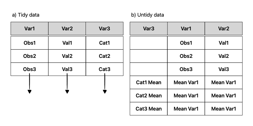
Tidy data has been a de facto approach to structure a dataset for easier analysis (Wickham 2014). A dataset is considered tidy if row is an observation, every column a variable. Visually, tidy data can be called rectangular (Figure Figure 6.1). Generally speaking, untidy data may contain summary rows, and is usually used for viewing versus computation. Wikipedia is a great place to search for examples of untidy data tables, or from user-provided collections.

Figure 6.1: Examples of tidy data (Panel a) and untidy data (Panel b)

Tidy data is actually just another name for Codd’s 3rd normal form, which is a term that comes from relational databases. It was first defined in 1971 by Edgar Codd, but has become more popular in recent years outside of the database world because of the popularity of the tidyverse packages in the R programming language ecosystem that expects data to be tidy. in this format. It is a form of data that not only is rectangular, but also aims to reduce data duplication and to allow for easy computation. True tidy data shares an incredible amount conceptually with the way that large relational databases are designed – in fact, R packages like dplyr can seamlessly connect to relational database servers using R syntax because the conceptual operations under the hood are nearly identical.

While tidy data is the aim, it shouldn’t be a necessary principle for data sharing and analysis in all cases. An insistence on tidy, “clean” data has troubled origins to statistics and the eugenics (D’Ignazio and Klein 2020). The accessibility of datasets is a good thing, but it also adds an extra onus for the end user to ensure the dataset is analyzed collaboratively, with findings connected back to the original owners. This is definitely connected to the contributor roles taxonomy that we will discuss in Chapter Chapter 22.

6.3.1 Spreadsheet data

Some strategies could be to randomly sample dataset rows or to switch to an alternative tool that is built to handle datasets that don’t fit into memory. Two examples are SQL for relational databases and streaming tools such as those commonly used on the Unix/Linux command line (grep/sed/awk). We discuss these more in Chapter XXX

Constraints on local computing

6.4

As a user you will need to decide if deciding to download the data from a server to your computer is worth it. Here are some considerations to decide if it is better to do analyses on servers where the data already are archived so the download/transfer step can be skipped.

Disk space: can your computer store the file?
random access memory (RAM): do you have a lot available, or are other processes using it?
CPU speed: can your computer handle complex calculations and manipulations to data
graphics processing (GPU): will you be able to visualize the data quickly
Network bandwidth: can the data be downloaded reasonably quickly? Disk speed (read/write speed)
Time needed to run analyses: can your computer efficiently run these analyses?

Ultimately is it going to be easier to bring the data to the compute or to bring the compute to the data?

6.5 Exercises

Search a particular subject on the Environmental Data Initiative Repository. Select two datasets that appear to have common themes. Are the two datasets standardized?