21.1 A discrete system
Let’s focus on an example that involves discrete populations. Moose are large animals (part of the deer family) weighing 1000 pounds that can be found in Northern Minnesota link. Here is a picture of a moose: link. While in the early 2000’s the population of the moose was 8000, recent estimates have the numbers at 3000, although that seems to have stabilized link
A starting model that describes their population dynamics is the discrete dynamical system:
\[\begin{equation} M_{t+1} = M_{t} + b \cdot M_{t} - d \cdot M_{t}, \tag{21.1} \end{equation}\]
where \(M_{t}\) is the population of the moose in year \(t\), and \(b\) the birth rate and \(d\) the death rate. This equation can be reduced down to \(M_{t+1}=r M_{t}\) where \(r=1+b-d\) is the net birth/death rate. This model states that the population of moose in the next year equals the current population, added to any fraction of births and taking away any deaths.
This discrete dynamical system is a little bit different from a continuous dynamical system, but can be simulated pretty easily by defining a function.
M0 <- 3000 # Initial population of moose
N <- 5 # Number of years we simulate

moose <- function(r) {
  out_moose <- array(M0, dim = N)
  for (i in 1:(N - 1)) {
    out_moose[i + 1] <- r * out_moose[i]
  }
  return(out_moose)
}
Notice how the function moose returns the current population of moose after \(N\) years with the net birth rate \(r\). Let’s take a look at the results for different values of \(r\) (Figure 21.1).
moose_rates <- tibble(
  years = 1:N,
  r0.4 = moose(0.4),
  r0.8 = moose(0.8),
  r1.1 = moose(1.1)
)


ggplot(data = moose_rates) +
  geom_line(aes(x = years, y = r0.4), color = "red") +
  geom_line(aes(x = years, y = r0.8), color = "blue") +
  geom_line(aes(x = years, y = r1.1), color = "green") +
  labs(
    x = "Years",
    y = "Moose"
  )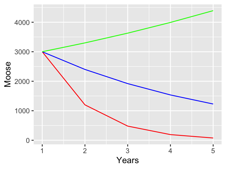
Figure 21.1: Simulation of the moose population with different birth rates.
Let’s remind ourselves of what is going on in the code.
out_moose <- tibble...creates a data frame that we can use for plotting. We call several different instances of themoosecode for different net birth rates. I’ve decided to label each of those instances with the value of the birth raterfor reference.- The command
geom_linemakes a line plot. Remember that we need to specify both the x (horizontal) and y (vertical) axes. I specified the different colors to distinguish the different birth rates.
Notice how for some values of \(r\) the population starts to decline, stay the same, or increase. Let’s analyze this system a little more. Just like with a continuous differential equation we want to look for solutions that are in steady state, or ones were the population is staying the same. In other words this means that \(M_{t+1}=M_{t}\), or \(M_{t}=rM_{t}\). If we simplify this expression this means that \(M_{t}-r M_{t}=0\), or \((r-1)M_{t}=0\). Assuming that \(M_{t}\) is not equal to zero, then this equation is consistent only when \(r=1\). This makes sense: we know \(r=1-b-d\), so the only way this can be one is if \(b=d\), or the births balance out the deaths.
Ok, so we found our equilibrium solution. However what is the general form of this solution to Equation (21.1)? Just like when we were solving continuous differential equations (Section 7 a starting point was that the solution was exponential. For discrete systems we will do the same, but this time we represent the solution as \(M_{t}=A\cdot v^{t}\), which is an exponential equation. Since we have \(M_{0}=3000\), then \(A=3000\). Using these values of \(M_{0}\) and \(A\) for Equation (21.1) we obtain the following:
\[\begin{equation} 100 \cdot v^{t+1} = r 3000 \cdot v^{t} \end{equation}\]
Our goal is to figure out a value for \(v\) that is consistent with this expression. Just like we did with continuous differential equations we can arrange the following equation, using the fact that \(v^{t+1}=v^{t}\cdot v\):
\[\begin{equation} 3000 v^{t} (v-r) = 0 \end{equation}\]
Since we assume \(v\neq 0\), the only possibility is if \(v=r\). Aha! Our general solution then is
\[\begin{equation} M_{t}=3000 r^{t} \end{equation}\]
We know that if \(r>1\) we have exponential growth exponential decay when \(r<1\) exponential decay, consistent with our results above.
There is some comfort here: just like in continuous systems we find the eigenvalues that determine the stability of the equilibrium solution. For discrete systems the stability is based on the eigenvalue relative to 1 (not 0) - so it is good to be aware of what type of system (discrete or continuous) you determining eigenvalues for! Now that we have an understanding of how this system works we can begin to look at stochasticity.