9.3 Connecting probabilities to linear regression

Now that we have made that small excursion into probablity, let’s start to return back to the linear regression problem. Another way to phrase this the linear regression problem studied in the last section is to examine the probability distribution of the model-data residual \(\epsilon\):

\[\begin{equation} \epsilon_{i} = y_{i} - f(x_{i},\vec{\alpha} ). \end{equation}\]

The approach with likelihood functions assumes a particular probability distribution on each residual. One common assumption is that the residual distribution is normal with mean \(\mu=0\) and standard deviation \(\sigma\) (which could be specified as measurement error, etc).

\[\begin{equation} L(\epsilon_{i}) = \frac{1}{\sqrt{2 \pi} \sigma} e^{-\epsilon_{i}^{2} / 2 \sigma^{2} }, \end{equation}\]

To extend this further across all measurement, we use the idea of independent, identically distributed measurements so the joint likelihood of all the residuals is the product of the likelihoods. The assumption of independent, identically distributed is is a common one. As a note of caution you should always evaluate if this is a valid assumption for more advanced applications.

\[\begin{equation} L(\vec{\epsilon}) = \prod_{i=1}^{N} \frac{1}{\sqrt{2 \pi} \sigma} e^{-\epsilon_{i}^{2} / 2 \sigma^{2} }, \end{equation}\]

We are making progress here, but in order to fully characterize the solution we need to specify the parameters \(\vec{\alpha}\). A simple redefining of the likelihood function where we specify the measurements (\(x\) and \(y\)) and parameters (\(\vec{\alpha}\)) is all we need:

\[\begin{equation} L(\vec{\alpha} | \vec{x},\vec{y} )= \prod_{i=1}^{N} \frac{1}{\sqrt{2 \pi} \sigma} \exp(-(y_{i} - f(x_{i},\vec{\alpha} ))^{2} / 2 \sigma^{2} ) \end{equation}\]

Now we have a function where the best parameter estimate is the one that optimizes the likelihood.

To return to our original linear regression problem (Figure 9.1, as a reminder we wanted to fit the function \(y=bx\) to the following set of points:

x	y
1	3
2	5
4	4
4	10

The likelihood \(L(\epsilon_{i}) ~ N(0,\sigma)\) characterizing these data are the following:

\[\begin{equation} L(b) = \left( \frac{1}{\sqrt{2 \pi} \sigma}\right)^{4} e^{-\frac{(3-b)^{2}}{2\sigma}} \cdot e^{-\frac{(5-2b)^{2}}{2\sigma}} \cdot e^{-\frac{(4-4b)^{2}}{2\sigma}} \cdot e^{-\frac{(10-4b)^{2}}{2\sigma}} \tag{9.1} \end{equation}\]

For the purposes of our argument here, we will assume \(\sigma=1\). Figure 9.9 shows a plot of the likelihood function \(L(b)\).

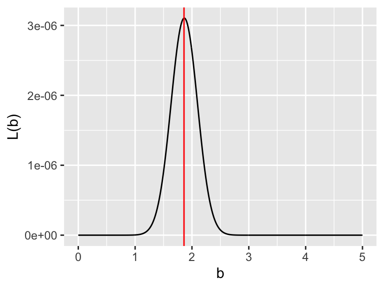
Figure 9.9: The likelihood function for the small dataset

Note that in Figure 9.9 the \(y\) values of \(L(b)\) are really small (this may be the case), the likelihood function is maximized at \(b=1.86\). An alternative to the small numbers in \(L(b)\) is to use the log likelihood (Equation (9.2)):

\[\begin{equation} \begin{split} \ln(L(\vec{\alpha} | \vec{x},\vec{y} )) &= N \ln \left( \frac{1}{\sqrt{2 \pi} \sigma} \right) - \sum_{i=1}^{N} \frac{ (y_{i} - f(x_{i},\vec{\alpha} )^{2}}{ 2 \sigma^{2}} \\ & = - \frac{N}{2} \ln (2) - \frac{N}{2} \ln(\pi) - N \ln( \sigma) - \sum_{i=1}^{N} \frac{ (y_{i} - f(x_{i},\vec{\alpha} )^{2}}{ 2 \sigma^{2}} \end{split} \tag{9.2} \end{equation}\]

In the homework you will be working on how to transform the likelihood function \(L(b)\) to the log-likelihood \(\ln(L(b))\).