26.1 The stochastic logistic model redux
Let’s go back to the logistic population model but re-written in a specific way:
\[\begin{equation} \frac{dx}{dt} = r x \left( 1 - \frac{x}{K} \right) = r x - \frac{rx^{2}}{K} \tag{26.1} \end{equation}\]
From Equation (26.1), we can obtain a change in the variable \(x\) (denoted as \(\Delta x\)) over \(\Delta t\) units by re-writing the differential equation in differential form:
\[\begin{equation} \Delta x = r x \Delta t - \frac{rx^{2}}{K} \Delta t \tag{26.2} \end{equation}\]
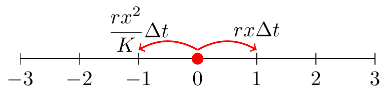
\(\displaystyle \Delta x = r x \Delta t - \frac{rx^{2}}{K} \Delta t\). Equation (26.2) is separated into two terms - one that increases the variable \(x\) (represented by \(r x \Delta t\), same units as \(x\)) and one that decreases the variable (represented by \(\displaystyle \frac{rx^{2}}{K} \Delta t\), same units as \(x\)). We will consider these changes as on a unit scale, organized via the following table:
| Outcome | Probability |
|---|---|
| \(\Delta x = 1\) (population change by 1) | \(r x \; \Delta t\) |
| \(\Delta x = -1\) (population change by -1) | \(\displaystyle \frac{rx^{2}}{K} \; \Delta t\) |
| \(\Delta x = 0\) (no population change) | \(\displaystyle 1 - rx \; \Delta t - \frac{rx^{2}}{K} \; \Delta t\) |
It also may be helpful to think of these changes on a random walk number line:
It may seem odd to think of the different outcomes (\(\Delta x\) equals 1, -1, or 1) as probabilities. Part of the reason why that formulation is useful is to apply concepts from probability theory. Let \(Y\) be a random variable with a finite number of finite outcomes \(\displaystyle y_{1},y_{2},\ldots ,y_{k}\) with probabilities \(\displaystyle p_{1},p_{2},\ldots ,p_{k}\), respectively, then the expected value \(\mu\) of \(Y\) is:
\[\begin{equation*} \mu = E[Y] = \sum_{i=1}^{k} y_{i}\,p_{i}=y_{1}p_{1}+y_{2}p_{2}+\cdots +y_{k}p_{k}. \end{equation*}\]
If we apply this definition to the random variable \(\Delta x\) we have:
\[\begin{equation} \begin{split} \mu = E[\Delta x] &= (1) \cdot \mbox{Pr}(\Delta x = 1) + (- 1) \cdot \mbox{Pr}(\Delta x = -1) + (0) \cdot \mbox{Pr}(\Delta x = 0) \\ &= (1) \cdot \left( r x \; \Delta t \right) + (-1) \frac{rx^{2}}{K} \; \Delta t \\ &= r x \; \Delta t - \frac{rx^{2}}{K} \; \Delta t \end{split} \tag{26.3} \end{equation}\]
Notice that the right hand side of Equation (26.3) is the same as the right hand side of the original differential equation (Equation (26.2)))!
Next let’s also calculate the variance of \(\Delta x\), defined for a discrete random variable:
\[\begin{equation*} \sigma^{2} = E[(Y - \mu)^{2}] = \sigma^{2}= E[Y^{2}] - (E[Y] )^{2}. \end{equation*}\]
\[\begin{equation} \begin{split} \sigma^{2} = E[(\Delta x)^{2}] - (E[\Delta x] )^{2} &= (1)^{2} \cdot \mbox{Pr}(\Delta x = 1) + (- 1)^{2} \cdot \mbox{Pr}(\Delta x = -1) + (0)^{2} \cdot \mbox{Pr}(\Delta x = 0) - (E[\Delta x] )^{2} \\ &= (1) \cdot \left( r x \; \Delta t \right) + (1) \frac{rx^{2}}{K} \; \Delta t - \left( r x \; \Delta t - \frac{rx^{2}}{K} \; \Delta t \right)^{2} \end{split} \end{equation}\]
Along with the computation of the variance, We are going to compute the variance to first order in \(\Delta t\). Because of that, we are going to assume that in \(\sigma^{2}\) any terms involving \((\Delta t)^{2}\) are small, or in effect negligible. While this is a huge simplifying assumption for the variance, but it is useful!
Doing these calcuations we have that \(\displaystyle \sigma^{2} = \left( r x \; \Delta t \right) + \frac{rx^{2}}{K} \; \Delta t\). Computing the mean and variance will help characterize the ensemble average. In addition the following random walk properties can be applied:
- Since \(\Delta x\) is the sum of many smaller changes we can apply the central limit theorem to characterize \(\Delta x\) as a normal random variable.
- To first order, we assume that \(\Delta x\) follows a probability distribution that is normal with mean \(\mu\) and variance \(\sigma^{2}\).
- The distribution for \(\Delta x\) can be expressed as \(\Delta x = \mu + \sigma Z\), where Z is random variable from a unit normal distribution (so in
Rwe would usernorm(1)). - We can simulate \(\Delta x\) as a Wiener process.
- Since \(\Delta x = x_{n+1}-x_{n}\), then we have \(x_{n+1} = x_{n} + \mu + \sigma Z\).
Notice how the last step provides a way to generate a solution trajectory to our differential equation. Cool! To simulate this stochastic process we will use the function birth_death_stochastic, which is set up in a similar way to euler_stochastic from Section 25. I will append _log to denote “logistic” for each of the parts
# Identify the birth and death parts of the DE:
birth_rate_log <- c(dx ~ r*x)
death_rate_log <-  c(dx ~ r*x^2/K)

# Identify the initial condition and any parameters
init_log <- c(x=3)  # Be sure you have enough conditions as you do variables.
parameters_log <- c(r=0.8, K=100)   # parameters: a named vector

# Identify how long we run the simulation
deltaT_log <- .05    # timestep length
time_steps_log <- 200   # must be a number greater than 1

# Identify the standard deviation of the stochastic noise
sigma_log <- 1

# Do one simulation of this differential equation
out_log <- birth_death_stochastic(birth_rate = birth_rate_log,
                             death_rate = death_rate_log,
                             init_cond = init_log,
                             parameters = parameters_log,
                             deltaT = deltaT_log,
                             n_steps = time_steps_log,
                             sigma = sigma_log)

# Plot out the solution
ggplot(data = out_log) +
  geom_line(aes(x=t,y=x))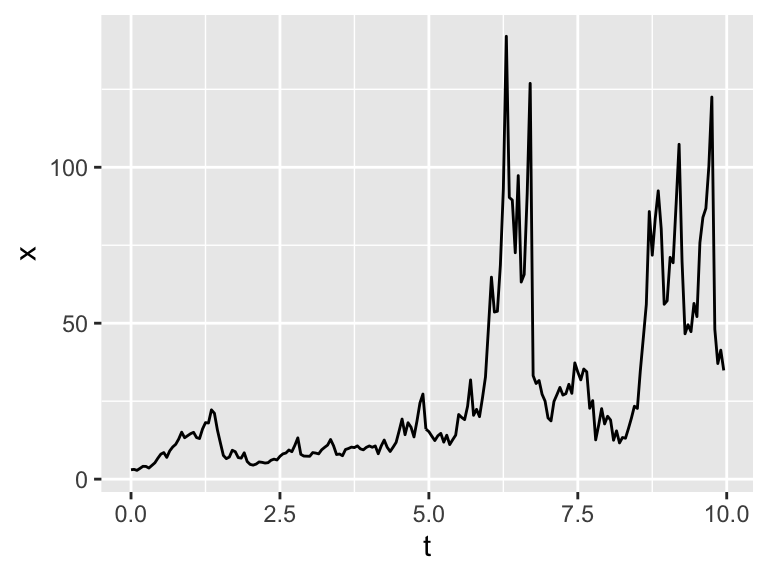
Figure 26.1: One realization of the logistic differential equation with stochastic variables.
Notice how the resulting spaghetti plot shows variation in the variables.
Making an ensemble average plot is also similar to how we computed them in Section 25:
# Many solutions
n_sims <- 100  # The number of simulations

# Compute solutions
logistic_sim_r <- rerun(n_sims) %>%
  set_names(paste0("sim", 1:n_sims)) %>%
  map(~ birth_death_stochastic(birth_rate = birth_rate_log,
                             death_rate = death_rate_log,
                             init_cond = init_log,
                             parameters = parameters_log,
                             deltaT = deltaT_log,
                             n_steps = time_steps_log,
                             sigma = sigma_log)
) %>%
  map_dfr(~ .x, .id = "simulation")


# Plot these all up together
  ggplot(data = logistic_sim_r) +
  geom_line(aes(x=t, y=x, color = simulation)) +
  ggtitle("Spaghetti plot for the logistic SDE") +
  guides(color="none")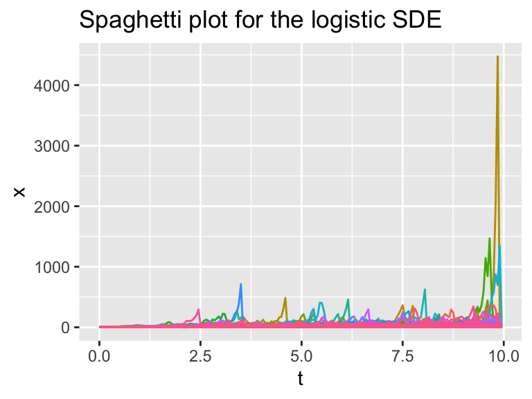
Figure 26.2: Several different realizations of the logistic SDE with stochasticity in the variables, along with the ensemble average plot.
  ### Summarize the variables
summarized_logistic_sim_r <- logistic_sim_r %>%
  group_by(t) %>%  # All simulations will be grouped at the same timepoint.
  summarise(x = quantile(x, c(0.25, 0.5, 0.75)), q = c("q0.025", "q0.5", "q0.975")) %>%
  pivot_wider(names_from = q, values_from = x)
## `summarise()` has grouped output by 't'. You can override using the `.groups` argument.### Make the plot
ggplot(data = summarized_logistic_sim_r) +
geom_line(aes(x = t, y = q0.5)) +
geom_ribbon(aes(x=t,ymin=q0.025,ymax=q0.975),alpha=0.2) +
ggtitle("Ensemble average plot for the logistic SDE")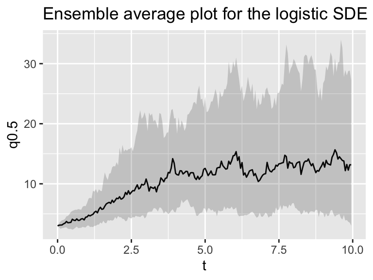
Figure 26.3: Several different realizations of the logistic SDE with stochasticity in the variables, along with the ensemble average plot.
Notice that as before the spaghetti and ensemble average plots are generated. While there are some simulations that may always be zero, in the ensemble the median resembles the (deterministic) solution to the logistic differential equation.
The types of stochastic processes we are describing in this section are called “birth-death” processes. Here is another way to think about Equation (26.2):
\[\begin{equation} \begin{split} r x \; \Delta t &= \alpha(x) \mbox{ (birth) }\\ \frac{rx^{2}}{K} \; \Delta t &= \delta(x) \mbox{ (death) } \end{split} \tag{26.4} \end{equation}\]
In this way we think of \(\alpha(x)\) in Equation (26.4) as a “birth process” and \(\delta(x)\) as a “death process.” When we computed the mean \(\mu\) and variance \(\sigma^{2}\) for Equation (26.2) we had \(\mu = \alpha(x)-\delta(x)\) and \(\sigma^{2}=\alpha(x)+\delta(x)\) (you should double check to make sure this is the case!). Here is an interesting fact: \(\mu = \alpha(x)-\delta(x)\) and \(\sigma^{2}=\alpha(x)+\delta(x)\) holds up for any differential equation where we have identified a birth or death process.