20.2 Bifurcations with systems of equations

As another example, let’s determine the behavior of solutions near the origin for the system of equations: \[\begin{equation} \frac{\vec{dx}}{dt} = \begin{pmatrix} 3 & b \\ 1 & 1 \end{pmatrix} \vec{x}. \tag{20.1} \end{equation}\]

Let’s take a look at the phase plane with solution curves.

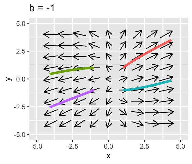
$Comparison of two phase planes for Equation \@ref(eq:b-bifurc-20)$

Figure 20.5: Comparison of two phase planes for Equation (20.1)

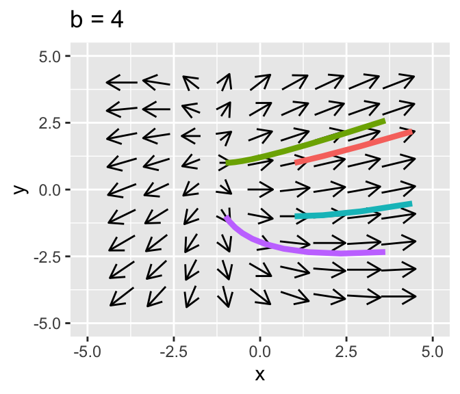
$Comparison of two phase planes for Equation \@ref(eq:b-bifurc-20)$

Figure 20.6: Comparison of two phase planes for Equation (20.1)

This equation has one free parameter $b$ that we will analyze using the trace determinant conditions developed in Section 19. Let’s call the matrix $A$, so the tr$(A)=4$ and $\det(A)=3-b$. Since the trace is always positive either it will be a saddle if the $\det(A)<0$, or when $3<b$. We have a unstable spiral when $3>b$ and $(\mbox{tr}(A))^2-4 \det(A)<0$, or when $4^2-4\cdot(3-b) = 16-12+4b = 4+4b<0$, which leads to $b<-1$. Notice this is a contradictory condition - we have already assumed $b>3$, so we will not have any unstable spirals.

To summarize, we have the following dynamics:

When $b<3$ the equilibrium solution will be a saddle.
When $b=3$ we will have an unstable solution.
When $b>3$ we will have a unstable node.

The benefit of a bifurcation diagram is that is provides a complete understanding of the dynamics of the system as a function of the parameters. In this section we examined one-parameter bifurcations (for example we looked the stability of the equilibrium solution as it depends on c or b), but bifurcations can also be extended further to two parameter bifurcation families, applying similar methods. In general the methods are similar to what we have done.