13.2 MCMC Parameter Estimation with a Differential Equation Model
Next let’s try parameter estimation with a differential equation model. What is different for this case is that we are given information about rate of change, so we need to first numerically solve the differential equation for a given parameter set and then compute the likelihood.
The example that we are going to use relates to land use management, in particular a coupled system between a resource (such as a national park) and the amount of visitors it receives (Sinay and Sinay 2006). The tourism model relies on two non-dimensonal scaled variables, \(R\) which is the amount of the resource (as a percentage) and \(V\) the percentage of visitors that could visit (also as a percentage):
\[\begin{equation} \begin{split} \frac{dR}{dt}&=R\cdot (1-R)-aV \\ \frac{dV}{dt}&=b\cdot V \cdot (R-V) \end{split} \tag{13.2} \end{equation}\]
Equation (13.2) has two parameters \(a\) and \(b\), which relate to how the resource is used up as visitors come (\(a\)) and how as the visitors increase, word of mouth leads to a negative effect of it being too crowded (\(b\)).
For this case we are going to use a pre-defined dataset of the number of resources and visitors to a national park as reported in Sinay and Sinay (2006) (Table 13.1) and plotted in Figure 13.3| time | visitors | resources |
|---|---|---|
| 0.0000000 | 0.0016667 | 0.9950 |
| 0.2833333 | 0.0046667 | 0.9860 |
| 0.3980000 | 0.0083333 | 0.9750 |
| 0.4513333 | 0.0150000 | 0.9550 |
| 0.4933333 | 0.0230000 | 0.9310 |
| 0.6553333 | 0.0238333 | 0.9285 |
| 0.6640000 | 0.0263330 | 0.9210 |
| 0.7280000 | 0.0321667 | 0.9035 |
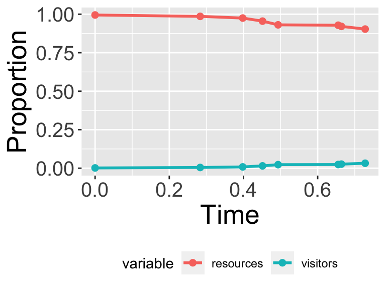
Figure 13.3: Scaled data on resources and visitors to a national park over time.
We can see that the data show as the visitors increase the percentage of the resources decrease. Perhaps from this limited dataset given we can estimate the parameters \(a\) and \(b\). We are going to assume that \(0 \leq a \leq 30\) and \(0 \leq b \leq 5\). We will need to implement this model in our code, which combines our knowledge of how we numerically solved differential equations in Section 4.
# Define the tourism model
tourism_model <- c(
  dRdt ~ resources * (1 - resources) - a * visitors,
  dVdt ~ b * visitors * (resources - visitors)
)

# Define the parameters that you will use with their bounds
tourism_param <- tibble(
  name = c("a", "b"),
  lower_bound = c(10, 0),
  upper_bound = c(30, 5)
)

# Define the initial conditions
tourism_init <- c(resources = 0.995, visitors = 0.00167)

deltaT <- .1 # timestep length
n_steps <- 15 # must be a number greater than 1

# Define the number of iterations
tourism_iter <- 1000

tourism_out <- mcmc_estimate(
  model = tourism_model,
  data = parks,
  parameters = tourism_param,
  mode = "de",
  initial_condition = tourism_init,
  deltaT = deltaT,
  n_steps = n_steps,
  iterations = tourism_iter,
)
Notice how mcmc_estimate has some additional arguments. Most importantly is the option mode, which de stands for differential equation. (The default mode is emp, or empirical model - like the phosphorous data set.) If the de mode is specified, then you also need to define defining the initial conditions (tourism_init), \(\Delta t\) (deltaT), and timesteps (n_steps).
Visualizing the data also is done with mcmc_visualize:
mcmc_visualize(
  model = tourism_model,
  data = parks,
  mcmc_out = tourism_out,
  mode = "de",
  initial_condition = tourism_init,
  deltaT = deltaT,
  n_steps = n_steps
)
Examining the parameter histograms (Figure 13.4) show \(b\) to be well-constrained. The histogram for \(a\) seems like it could be well-constrained - but we may need to run more iterations to confirm this.
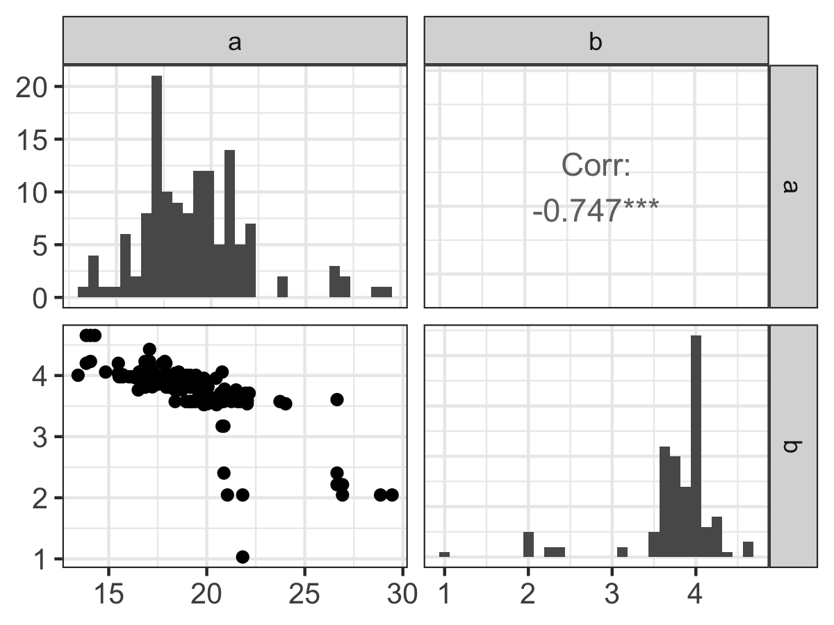
Figure 13.4: Pairwise parameter histogram of MCMC parameter estimation results for Equation (13.2)
The model results and confidence intervals show good agreement to the data (Figure 13.5), also confirming that as visitors increase, the resources in the national park will decrease due to overuse.
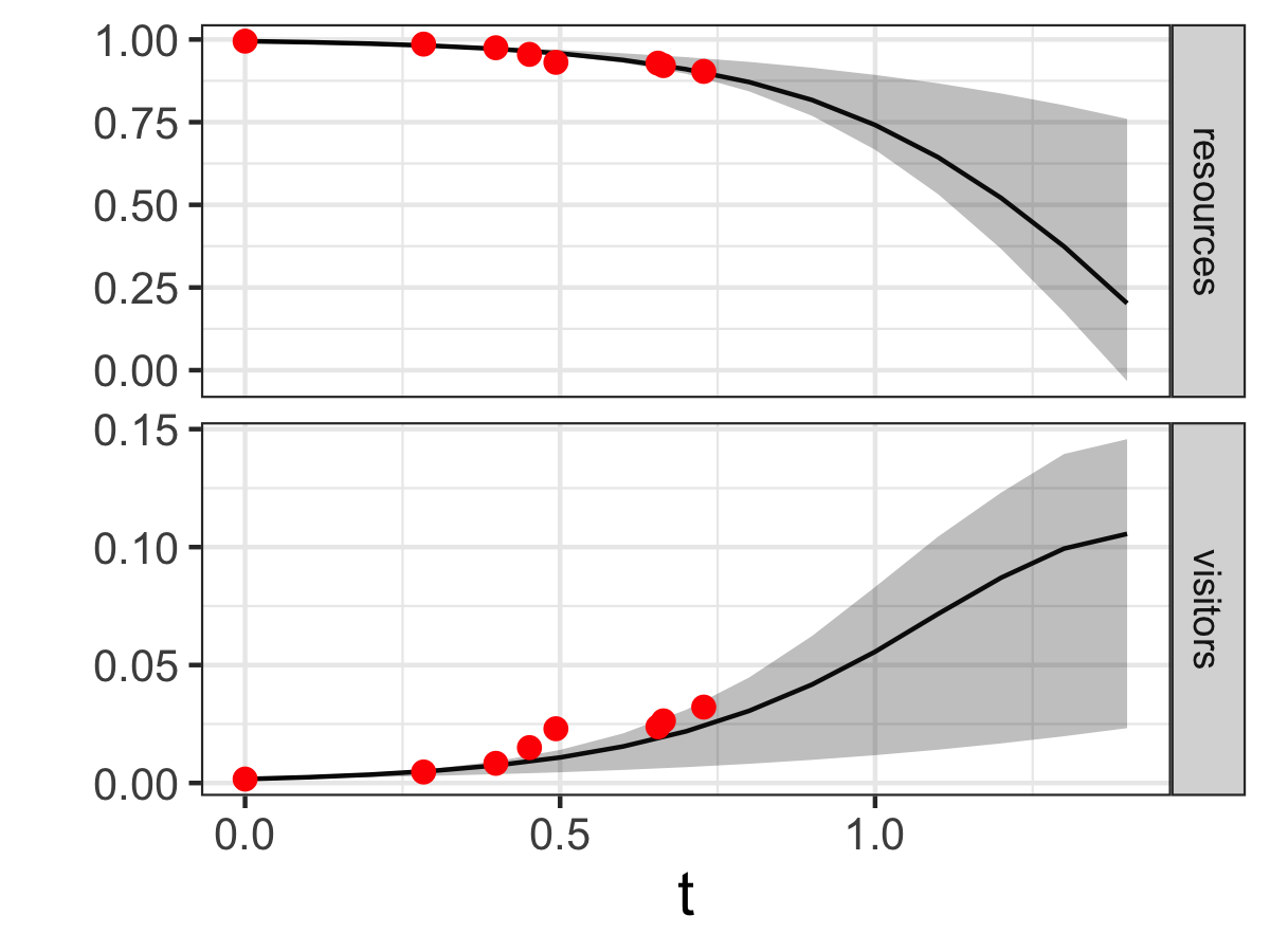
Figure 13.5: Ensemble output results from the MCMC parameter estimation for Equation (13.2).