4.3 Euler’s method applied to systems

Now that we have some experience with Euler’s method, let’s see how we can apply the function euler to a system of differential equations. Here is a sample code that shows the dynamics for the Lotka-Volterra equations, as studied in Section 3:

\[\begin{equation} \begin{split} \frac{dH}{dt} &= r H - bHL \\ \frac{dL}{dt} &= e b H L - dL \end{split} \tag{4.1} \end{equation}\]

We are going to use Euler’s method to solve this differential equation. Similar to the previous example we will need to determine the f

# Define the rate equation:
lynx_hare_eq <- c(
  dHdt ~ r * H - b * H * L,
  dLdt ~ e * b * H * L - d * L
)


# Define the parameters (as a named vector)
lynx_hare_params <- c(r = 2, b = 0.5, e = 0.1, d = 1) # parameters: a named vector

# Define the initial condition (as a named vector)
lynx_hare_init <- c(H = 1, L = 3)

# Define deltaT and the time steps:
deltaT <- 0.05 # timestep length
timeSteps <- 200 # must be a number greater than 1

# Compute the solution via Euler's method:
out_solution <- euler(system_eq = lynx_hare_eq,
                      parameters = lynx_hare_params,
                      initial_condition = lynx_hare_init,
                      deltaT = deltaT,
                      n_steps = n_steps
                      )

# Make a plot of the solution, using different colors for lynx or hares.
ggplot(data = out_solution) +
  geom_line(aes(x = t, y = H), color = "red") +
  geom_line(aes(x = t, y = L), color = "blue") +
  labs(
    x = "Time",
    y = "Lynx (red) or Hares (blue)"
  )

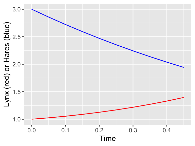
Figure 4.4: Euler's method solution for Lynx-Hare system

This example is structured similarly as a single variable differential equation, with some key changes:

• The variable lynx_hare_eq is now a vector, with each entry one of the rate equations.
• We need to identify both variables in their initial condition.
• Most importantly, Equation (4.1) has parameters, which we define as a named vector lynx_hare_params <- c(r = 2, b = 0.5, e = 0.1, d = 1) that we pass through to the command euler with the option parameters. If your equation does not have any parameters you do not need to worry about specifying this input.
• We plot both solutions together at the end, or you can make two separate plots. Remember that you can choose the color in your plot.

Thankfully the euler code is pretty easy to adapt for systems of equations!