25.3 Adding stochasticity to parameters

Now that we have seen an example in adding stochasticity to the logistic equation, we can also parameters of the differential equation to be stochastic. For example, let’s say that the growth rate \(r\) in the logistic equation is subject to stochastic effects. How we would implement this by replacing \(r\) with \(r + \mbox{ Noise }\):

\[\begin{equation} dx = (r + \mbox{ Noise } ) \; x \left(1 - \frac{x}{K} \right) \; dt, \end{equation}\]

Now what we do is separate out the terms that are multiplied by “Noise” - they will form the stochastic part of the differential equation. The terms that aren’t multipled by “Noise” form the deterministic part of the differential equation:

\[\begin{equation} dx = r x \left(1 - \frac{x}{K} \right) \; dt + x \left(1 - \frac{x}{K} \right) \mbox{ Noise } \; dt, \end{equation}\]

So we have the following, writing \(\mbox{ Noise } \; dt = dW(t)\): \[\begin{align*} \mbox{Deterministic part: } & rx \left(1 - \frac{x}{K} \right) \; dt \\ \mbox{Stochastic part: } & x \left(1 - \frac{x}{K} \right) dW(t) \end{align*}\]

There are a few things to notice here. First, the deterministic part of the differential equation is what we would expect without noise added. Second, notice how the stochastic part of the differential equation changed. Let’s take a look at the simulations with the Euler-Maruyama method, denoting the deterministic and stochastic parts as deterministic_logistic_r and stochastic_logistic_r respectively:

# Identify the deterministic and stochastic parts of the DE:
deterministic_logistic_r <- c(dx ~ r*x*(1-x/K))
stochastic_logistic_r <-  c(dx ~ x*(1-x/K))

# Identify the initial condition and any parameters
init_logistic <- c(x=3)  # Be sure you have enough conditions as you do variables. 
logistic_parameters <- c(r=0.8, K=100)   # parameters: a named vector

# Identify how long we run the simulation
deltaT_log <- .05    # timestep length
timeSteps_log <- 200   # must be a number greater than 1

# Identify the standard deviation of the stochastic noise
sigma_log <- 1

# Do one simulation of this differential equation
logistic_out <- euler_stochastic(deterministic_rate = deterministic_logistic_r,
                             stochastic_rate = stochastic_logistic_r,
                             init_cond = init_logistic,
                             parameters = logistic_parameters,
                             deltaT = deltaT_log,
                             n_steps = timeSteps_log,
                             sigma = sigma_log)

# Plot out the solution
ggplot(data = logistic_out) +
  geom_line(aes(x=t,y=x))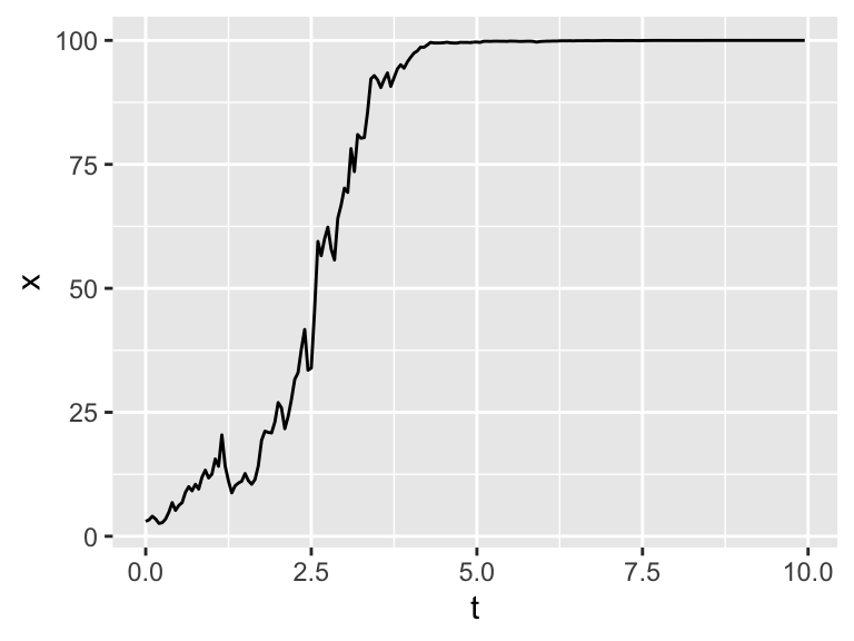

Figure 25.4: One realization of the logistic differential equation with stochasticity in the parameter r.

As we did before, we can run multiple iterations of this stochastic process. We will also compute and plot the ensemble average.

# Many solutions
n_sims <- 100  # The number of simulations

# Compute solutions
logistic_run_r <- rerun(n_sims) %>%
  set_names(paste0("sim", 1:n_sims)) %>%
  map(~ euler_stochastic(deterministic_rate = deterministic_logistic_r,
                             stochastic_rate = stochastic_logistic_r,
                             init_cond = init_logistic,
                             parameters = logistic_parameters,
                             deltaT = deltaT_log,
                             n_steps = timeSteps_log,
                             sigma = sigma_log)
) %>%
  map_dfr(~ .x, .id = "simulation")


# Plot these all up together
  ggplot(data = logistic_run_r) +
  geom_line(aes(x=t, y=x, color = simulation)) +
  ggtitle("Spaghetti plot for the logistic SDE") +
  guides(color="none")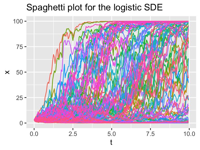

Figure 25.5: Several different realizations of the logistic SDE with stochasticity in the parameter r, along with the ensemble average plot.

  ### Summarize the variables
summarized_logistic_r <- logistic_run_r %>%
  group_by(t) %>%  # All simulations will be grouped at the same timepoint.
  summarise(x = quantile(x, c(0.25, 0.5, 0.75)), q = c("q0.025", "q0.5", "q0.975")) %>%
  pivot_wider(names_from = q, values_from = x)

## `summarise()` has grouped output by 't'. You can override using the `.groups` argument.

### Make the plot
ggplot(data = summarized_logistic_r) +
  geom_line(aes(x = t, y = q0.5)) +
  geom_ribbon(aes(x=t,ymin=q0.025,ymax=q0.975),alpha=0.2) +
  ggtitle("Ensemble average plot for the logistic SDE")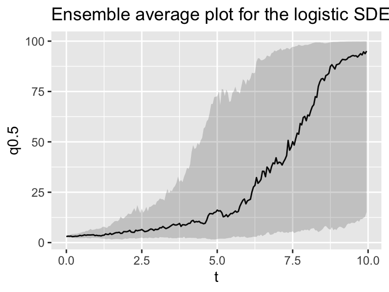

Figure 25.6: Several different realizations of the logistic SDE with stochasticity in the parameter r, along with the ensemble average plot.

Wow! Adding in stochasticity to the parameters changes things. Notice how the dynamics are different - there is a lot more variability in how quickly the solution rises to the steady state of \(K=100\).