4.4 More refined numerical solvers

Perhaps in the course of working with Euler’s method you encounter a differential equation that produces some nonsensible results. Take for example the following which is the implementation of our quarantine model:

quarantine_eq <- c(
  dSdt ~ -k * S * I,
  dIdt ~ k * S * I - beta * I
)


deltaT <- .1 # timestep length
timeSteps <- 15 # must be a number greater than 1

quarantine_parameters <- c(k = .05, beta = .2) # parameters: a named vector

quarantine_init <- c(S = 300, I = 1) # Be sure you have enough conditions as you do variables.

# Compute the solution via Euler's method:
out_solution <- euler(system_eq = quarantine_eq,
                      parameters = quarantine_parameters,
                      initial_condition = quarantine_init,
                      deltaT = deltaT,
                      n_steps = n_steps
                      )


ggplot(data = out_solution) +
  geom_line(aes(x = t, y = S), color = "red") +
  geom_line(aes(x = t, y = I), color = "blue") +
  labs(
    x = "Time",
    y = "Susceptible (red) or Infected (blue)"
  )

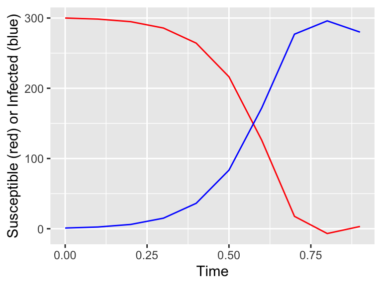
Figure 4.5: Surprising results with Euler’s method.

You may notice the solution for \(S\) wiggles around \(t=0.75\) and is negative. This is concerning because we know there can’t be negative people! This requires a little more investigation.

If we take a look at \(t=0.75\) the value for \(S \approx 1\) and the value for \(I \approx 280\). If we let \(k=0.05\) and \(\beta=0.2\), this means that \(\displaystyle \frac{dS}{dt}=-14\) and \(\displaystyle \frac{dI}{dt}=-42\). The values of \(S\) and \(I\) are both decreasing! We know that our Euler’s method update is one where the new value is the old value plus any change. So the new value for \(S = 1 -14\cdot 0.1 = -0.4\). Mathematically, Euler’s method working correctly, but we know realistically that neither \(S\) or \(I\) can be negative.

In turns out that this can easily be overcome. While Euler’s method is useful, it does quite poorly in cases where the solution is changing rapidly - or we might need to make some smaller step sizes.

Another way to remedy this is to use a higher order solver, and one such method is called the Runge-Kutta Method. If you take a course in numerical analysis you might study these, but for the moment you see the difference between the Runge-Kutta solver implemented in the demodelr package, which by all intents and purposes is replaces the command euler with rk4:

quarantine_eq <- c(
  dSdt ~ -k * S * I,
  dIdt ~ k * S * I - beta * I
)


deltaT <- .1 # timestep length
timeSteps <- 15 # must be a number greater than 1

quarantine_parameters <- c(k = .05, beta = .2) # parameters: a named vector

quarantine_init <- c(S = 300, I = 1) # Be sure you have enough conditions as you do variables.

# Compute the solution via a Runge-Kutta method:
out_solution <- rk4(system_eq = quarantine_eq,
                    parameters = quarantine_parameters,
                    initial_condition = quarantine_init,
                    deltaT = deltaT,
                    n_steps = n_steps
                    )


ggplot(data = out_solution) +
  geom_line(aes(x = t, y = S), color = "red") +
  geom_line(aes(x = t, y = I), color = "blue") +
  labs(
    x = "Time",
    y = "Susceptible (red) or Infected (blue)"
  )

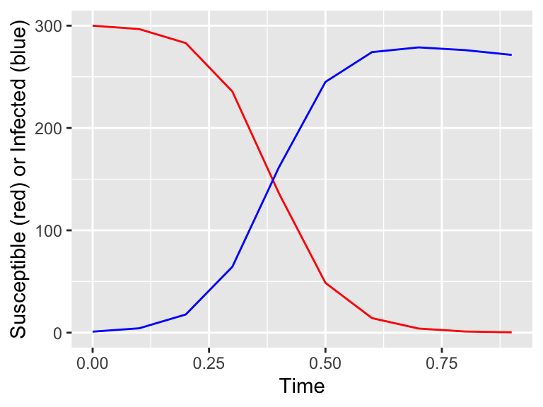
Figure 4.6: Better results with the Runge-Kutta method.

So what is going on here? Briefly, the differences between the two methods have to do with the error in the numerical method. The error is quantified as the difference between the actual solution and the numerical solution. Euler’s method has an error on the order of the stepsize \(\Delta t\), whereas the Runge-Kutta method has an error of \((\Delta t)^4\). For this example, the error in Euler’s method is 0.1 (\(\Delta t = .1\)), but for the Runge-Kutta method it is 0.0001 (\((\Delta t)^{4} =.0001\)). The error is noticeably different! While we can improve Euler’s method by taking a smaller timestep - BUT that means we need a larger number of steps \(N\) - which may take more computational time.

Does this discussion sound familiar? Perhaps you examined similar when you took calculus and studied Riemann sums to approximate the area underneath a curve (left sum, right sum, trapezoid, midpoint). It turns out that these two problems are closely related. Numerical analysis is a great field of study to examine these topics and others!

Moving ahead, I might switch between Euler’s method or the Runge-Kutta method when solving a differential equation. Thankfully the bulk of the work is “under the hood” - the setup will be the same for both!