26.4 Exercises
group_by(name,t) to begin summarizing our variables. Modify the code so you apply group_by(t,name) and generate the ensemble plot. Do you receive a similar result?
Exercise 26.4 For the logistic differential equation consider the following splitting of \(\alpha(x)\) and \(\delta(x)\):
\[\begin{equation} \begin{split} \alpha(x) &= rx + \frac{rx^{2}}{2K} \\ \delta(x) &= \frac{rx^{2}}{2K} \end{split} \end{equation}\]
Simulate this SDE using the same values of parameters for the logistic example and compare your results.
Exercise 26.5 (Inspired by Logan and Wolesensky (2009)) Let \(R(t)\) denote the rainfall at a location at time \(t\), which is a random process. Assume that probability of the change in rainfall from day \(t\) to day \(t+\Delta t\) is the following:
| change | probability |
|---|---|
| \(\Delta R = \rho\) | \(\lambda \Delta t\) |
| \(\Delta R = 0\) | \(1- \lambda \Delta t\) |
- With this information, compute E[\(\Delta R\)] and variance of \(\Delta R\).
- Simulate this stochastic process. Use \(R(0)=0\) and run 500 simulations of this stochastic process. Set \(\lambda \rho = 18\) and \(\sqrt{ \lambda \rho^{2}}=16\).
Exercise 26.6 Consider the following model for zombie population dynamics (Smith? 2014):
\[\begin{equation} \begin{split} \frac{dS}{dt} &=-\beta S Z - \delta S \\ \frac{dZ}{dt} &= \beta S Z + \xi R - \alpha SZ \\ \frac{dR}{dt} &= \delta S+ \alpha SZ - \xi R \end{split} \end{equation}\]
- Determine the birth and death terms for the zombie model so that you could encode this as a birth/death process:
- Birth part for \(\displaystyle \frac{dS}{dt}\):
- Death part for \(\displaystyle \frac{dS}{dt}\):
- Birth part for \(\displaystyle \frac{dZ}{dt}\):
- Death part for \(\displaystyle\frac{dZ}{dt}\):
- Birth part for \(\displaystyle \frac{dR}{dt}\):
- Death part for \(\displaystyle \frac{dR}{dt}\):
- Use
birth_death_stochasticto perform 500 simulations of this stochastic differential equation. Please assume the following values of the parameters and stochastic method:
- \(\sigma = 0.004\)
- \(\Delta t= 0.5\).
- Timesteps: 200.
- \(\beta = 0.0095\), \(\delta = 0.0001\) ,\(\xi = 0.1\), \(\alpha = 0.005\).
- Initial condition: \(S(0)=499\), \(Z(0)=1\), \(R(0)=0\).
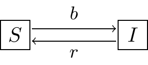
Figure 26.8: The \(SIS\) model
Exercise 26.8 (Inspired by Logan and Wolesensky (2009)) An \(SIS\) model is one where susceptibles \(S\) become infected \(I\), and then after recovering from an illness, become susceptible again. The schematic representing this is shown in Figure 26.8. While you can write this as a system of differential equations, assuming the population size is constant \(N\) we have the following differential equation:
\[\begin{equation} \frac{dI}{dt} = b(N-I) I - r I \end{equation}\]
- Identify \(\alpha(I)\) and \(\delta(I)\) for this model.
- Assuming \(N=1000\), \(r=0.01\), and \(b=0.005\), \(I(0)=1\), simulate this differential equation over two weeks with \(\Delta t = 0.1\). Show the plot of your result.
Exercise 26.9 Consider the equation \[\begin{equation*} \Delta x = \alpha(x) \; \Delta t - \delta(x) \; \Delta t \end{equation*}\]
If we consider \(\Delta x\) to be a random variable, show that the expected value \(\mu\) equals \(\alpha(x) \; \Delta t - \delta(x) \; \Delta t\) and the variance \(\sigma^{2}\), to first order, equals \(\alpha(x) \; \Delta t + \delta(x) \; \Delta t\).