21.2 Environmental Stochasticity
It may be the case that environmental effects drastically change the net birth rate from one year to the next. For example it is known that in snowy winters the net birth rate changes because it is difficult to find food (Carroll 2013). For our purposes, let’s say that in snowy winters \(r\) changes from \(1.1\) to \(0.7\). This would be a pretty drastic effect on the system - as one case is associated with exponential growth and the other exponential decay.
Because the years when snowy winters occur is random, we need to account for this in our model. One way is to create a conditional statement based on the probability of the moose to adjust to a deep snowpack in a given year. We will define this probability to be on a scale from 0 to 1, where 0 means the moose cannot adjust to a deep snowpack, and 1 they are able to adjust to a deep snowpack. How we implement that is writing a function that draws a uniform random number each year and adjusting the birth rate:
# We use the snowfall_rate  as an input variable

moose_snow <- function(snowfall_prob) {
  out_moose <- array(M0, dim = N)
  for (i in 1:(N - 1)) {
    r <- 1.1 # Normal net birth rate
    if (runif(1) > snowfall_prob) {
      r <- 0.7 # Decreased birth rate
    }
    out_moose[i + 1] <- r * out_moose[i]
  }
  return(out_moose)
}
Let’s take a look at some solutions for different realizations of the moose population over time when the probability to adjust to the snowfall rate varies.
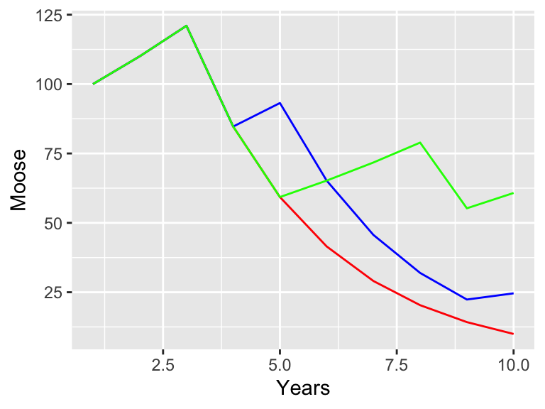
Figure 21.2: Moose populations with different probability of adjusting to deep snowpacks.
Run the above code on your computer. Do you obtain the same result? I hope not! We are drawing random numbers for each year, so you should have different trajectories. While this may seem like a problem, one key thing that we will learn in Section 22 is when we compute multiple simulations and then compute an ensemble average we see patterns in the results.
As you can see when the probability of adjusting to deep snowpacks is very high (\(p = 0.75\)), the population continues exponentially. If that probability is lower, it can still increase, but one bad year does knock the population down.
The moose example introduced how random effects into the dynamical system. Both contexts (environmental or demographic stochasticity) affected the net reproduction rate \(r\), but in different ways. The important lesson is that the type of stochasticity matters just as much as how it is implemented.