6.1 Model redux: flu with quarantine

In Section 1 we studied the following model for the flu as a coupled system of equations:

\[\begin{equation} \begin{split} \frac{dS}{dt} &= -kSI \\ \frac{dI}{dt} &= kSI \\ \end{split} \tag{6.1} \end{equation}\]

In this scenario we are also going to consider that those who are infected are quarantined, proportional to the number infected, according to the following schematic:

Which gives us the following system of equations: \[\begin{equation} \begin{split} \frac{dS}{dt} &= -kSI \\ \frac{dI}{dt} &= kSI - \beta I \end{split} \tag{6.2} \end{equation}\]

To find the equilibrium solutions we want to find values of $S$ and $I$ where the rates $\displaystyle \frac{dS}{dt}$ and $\displaystyle \frac{dI}{dt}$ are both zero. This can be done by algebraically solving the system of equations:

\[\begin{equation} \begin{split} 0 &= -kSI \\ 0 &= kSI - \beta I \end{split} \end{equation}\]

Let’s examine the first equation ($0 = -kSI$), which we can see is consistent when either $S=0$ and $I=0$. These give us two options, which we then use in the second equation ($0 = kSI - \beta I$). When $S=0$, then $0 = k\cdot 0 \cdot I - \beta I \rightarrow 0 = -\beta I$, which is consistent when $I=0$. So $(S_{*},I_{*}) = (0,0)$ is one equilibrium solution. The other case when $I=0$ gives us that any value of $S$ would be an equilibrium solution. Can you explain why?

Equation (6.2) and its equilibrium solutions are an interesting example. We call the equations $S=0$ and $I=0$ when $\displaystyle \frac{dS}{dt}=0$ as nullclines for $S$. In a similar manner, the equations in $S$ and $I$ when $\displaystyle \frac{dI}{dt}=0$ are called nullclines for $I$. Let’s try to determine formulas for these equations:

\[\begin{equation} \begin{split} 0 &= kSI-\beta I \\ 0 &= I\cdot (kS - \beta ) \end{split} \end{equation}\]

Because the last equation is factored as a product, nullclines for $I$ are either $I=0$ or $\displaystyle S = \frac{\beta}{k}$.

Nullclines are not equilibrium solutions by themselves - it is the intersection of two different nullclines that determine equilibrium solutions. Figure 6.1 shows the nullclines in the $S-I$ plane (since we have two equations), with $S$ on the horizontal axis and $I$ on the vertical axis.

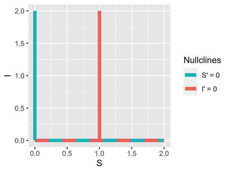
$Nullclines for Equation \@ref(eq:flu-quarantine). To generate the plot we assumed $\beta=1$ and $k=1$$

Figure 6.1: Nullclines for Equation (6.2). To generate the plot we assumed $\beta=1$ and $k=1$

A key thing to note is that where two different nullclines cross is an equilibrium solution to the system of equations. This means that both $\displaystyle \frac{dS}{dt}$ and $\displaystyle \frac{dI}{dt}$ are zero at this point. Examining Figure 6.1, there are three possibilities:

There is an equilibrium solution at $S=0$ and $I=0$ (otherwise known as the origin). This equilibrium solution makes biological sense: if there is nobody susceptible or infected there are no flu cases (everyone is perfectly healthy - yay!) .
The entire horizontal axis is an equilibrium solution because $I=0$, which makes both $\displaystyle \frac{dS}{dt}$ and $\displaystyle \frac{dI}{dt}$ both zero. There is a practical interpretation of this nullcline - whenever $I=0$, meaning there are no infected people around, so infection cannot occur.
There is also a third possibility where the vertical line at $S=1$ crosses the horizontal axis ($S=1$, $I=0$), but that also falls under the second equilibrium solution.

Now that we have identified our nullclines and equilibrium solutions, we will add additional context with the flow of the solution.

6.1.1 Adding context to our phase plane: slope fields

Let’s go back to the idea of a phase plane, but this time we are going to add more context to our nullcline graph by evaluating different values of $S$ and $I$ into our system of equations and plot the slope field.

Table 6.1 evaluates the derivatives $\displaystyle \frac{dS}{dt}$ and $\displaystyle \frac{dI}{dt}$ in Equation (6.2) for different values of $S$ and $I$.

Table 6.1: Values of $\displaystyle \frac{dS}{dt}$ and $\displaystyle \frac{dI}{dt}$ for the flu with quarantine model.
S	I	dS_dt	dI_dt
0.0000000	0.0000000	0.0000000	0.0000000
0.4444444	0.4444444	-0.1975309	-0.2469136
0.8888889	0.8888889	-0.7901235	-0.0987654
1.3333333	1.3333333	-1.7777778	0.4444444
1.7777778	1.7777778	-3.1604938	1.3827160
2.2222222	2.2222222	-4.9382716	2.7160494
2.6666667	2.6666667	-7.1111111	4.4444444
3.1111111	3.1111111	-9.6790123	6.5679012
3.5555556	3.5555556	-12.6419753	9.0864198
4.0000000	4.0000000	-16.0000000	12.0000000

Notice how the different values of $\displaystyle \frac{dS}{dt}$ and $\displaystyle \frac{dI}{dt}$ at each of the $S$ and $I$ values. We can plot each of the coordinate pairs of $\displaystyle \left( \frac{dS}{dt}, \frac{dI}{dt} \right)$ as a vector in the $(S,I)$ plane. We associate $\displaystyle \frac{dS}{dt}$ with left-right motion, so positive $\displaystyle \frac{dS}{dt}$ means pointing to the right. Likewise, we associate $\displaystyle \frac{dI}{dt}$ with up-down motion, so positive $\displaystyle \frac{dI}{dt}$ means the vector points up. At the point $(S,I)=(1,1)$, we have an arrow that points directly to the west because and $\displaystyle \frac{dI}{dt} < 0$ and $\displaystyle \frac{dI}{dt} =0$. Continuing on in this manner, by sequentially sampling points in the $(S,I)$ plane we get a vector field plot (Figure 6.2), superimposed with the nullclines.

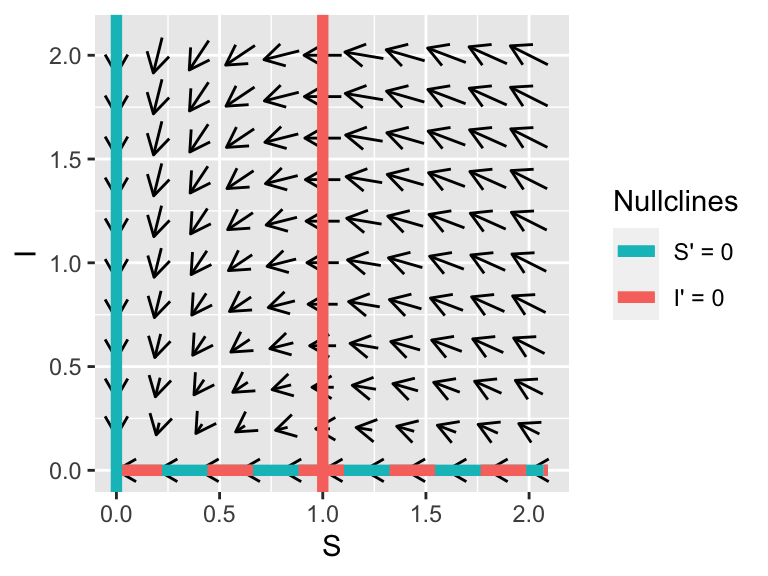
$Phaseplane for Equation \@ref(eq:flu-quarantine). To generate the plot we assumed $\beta=1$ and $k=1$$

Figure 6.2: Phaseplane for Equation (6.2). To generate the plot we assumed $\beta=1$ and $k=1$

6.1.2 Motion around the nullclines

We can also extend the motion around the nullclines to investigate the stability of an equilbrium solution. With a one dimensional differential equation we used a number line to quantify values where the solution is increasing / decreasing. The problem with several differential equations is that the notion of “increasing” or “decreasing”" becomes difficult to understand - there is an additional degree of freedom! Simply put, in a plane you can move left/right or up/down. The benefit for having nullclines is that they isolate the motion in one direction. When $\displaystyle \frac{dS}{dt}=0$ the only allowed motion is up and down; when $\displaystyle \frac{dI}{dt}=0$ the only allowed motion is left and right.

In general for a two dimensional system: - When a horizontal axis variable has a nullcline, the only allowed motion is up/down. - When a vertical axis variable has a nullcline, the only motion is up/down.

Applying this knowledge to Equation (6.2), if we choose points where $I'=0$ then we know that the only motion is to the left and the right because $S$ can still change along that curve. If we choose points where $S'=0$ then we know that the only motion is to the up/down because $I$ can still change along that curve (Figure 6.3).

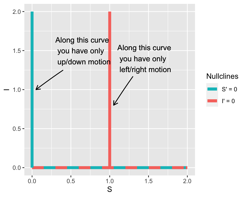
$Nullclines for Equation \@ref(eq:flu-quarantine) with context on the direction of the motion.$

Figure 6.3: Nullclines for Equation (6.2) with context on the direction of the motion.