7.2 Integrating factors

One model that we have looked at is the the \(SI\) model where the spread of the disease is proportional to the number infected:

\[\begin{equation} \frac{dI}{dt} = .03(1000-I) = 30 - .03I \tag{7.1} \end{equation}\]

While this differential equation can be solved via separation of variables, let’s try a different approach as an illustration of another useful technique. First let’s write the terms involving \(I\) on one side of the equation:

\[\begin{equation} \frac{dI}{dt} + .03I = 30. \end{equation}\]

What we are going to do is multiply both sides of this equation by \(e^{.03t}\) (I’ll explain more about that later):

\[\begin{equation} \frac{dI}{dt} \cdot e^{.03t} + .03I \cdot e^{.03t} = 30 \cdot e^{.03t} \end{equation}\]

Hmmm - this seems like we are making our equation harder to solve, doesn’t it? However the left hand side is actually the derivative of the expression \(I \cdot e^{kt}\)! Let’s take a look:

\[\begin{equation} \frac{d}{dt} \left( I \cdot e^{.03t} \right) = \frac{dI}{dt} \cdot e^{.03t} + I \cdot .03 e^{.03t} \end{equation}\]

This derivative is courtesy of the product rule from calculus. Ok, so what does this do to the differential equation? Well, by re-writing the differential equation as a derivative and integrating:

\[\begin{equation} \begin{split} \frac{d}{dt} \left( I \cdot e^{.03t} \right) &= 30 \cdot e^{.03t} \rightarrow \\ \int \frac{d}{dt} \left( I \cdot e^{.03t} \right) \; dt &= \int 30 \cdot e^{.03t} \; dt \rightarrow \\ I \cdot e^{.03t} &= 30 \cdot e^{.03t} + C \end{split} \end{equation}\]

Notice how by writing the left hand side in terms of the product rule and integrating we could find the solution. We added the \(+C\) to the right hand side. All that is left to do is to solve in terms of \(I(t)\) by dividing by \(e^{kt}\). We will label this solution \(I_{1}(t)\):

\[\begin{equation} I_{1}(t) = 1000 + Ce^{-.03t} \tag{7.2} \end{equation}\]

Cool! The function \(f(t)=e^{.03t}\) is called an integrating factor.

To see what is meant by that, let’s try one more example.

Example 7.1 Modifying Equation (7.1), now let’s assume that the rate of infection is time dependent, or \(k(t) = .03t\). Apply the method of integrating factors to determine a solution to this differential equation.

Solution. How this would work in practice is that initially (at \(t=0\)) there is no infection, but the infection rate increases as time goes on.

Our differential equation in this case is:

\[\begin{equation*} \frac{dI}{dt} + .03 t \cdot I = 30 t. \end{equation*}\]

So if we want to write the left hand side as a product, what we will do is multiply the entire differential equation by \(\displaystyle e^{\int .03t \; dt} = e^{ 0.015 t^{2}}\) This term is called the integrating factor:

\[\begin{equation} \frac{dI}{dt} \cdot e^{ 0.015 t^{2}} + .03 t \cdot I \cdot e^{0.015 t^{2}} = 30 t \cdot e^{0.015 t^{2}} \end{equation}\]

First we rewrite the left hand side using the product rule: \[\begin{equation} \frac{dI}{dt} \cdot e^{ 0.015 t^{2}} + .03 t \cdot I \cdot e^{0.015 t^{2}} = \frac{d}{dt} \left( I \cdot e^{0.015 t^{2}} \right). \end{equation}\]

Now we can integrate this equation with the product rule in reverse:

\[\begin{equation} \begin{split} \frac{d}{dt} \left( I \cdot e^{0.015 t^{2}} \right) &= 30 t \cdot e^{0.015 t^{2}} \rightarrow \\ \int \frac{d}{dt} \left( I \cdot e^{0.015 t^{2}} \right) \; dt &= \int 30t \cdot e^{0.015 t^{2}} \; dt \rightarrow \\ I \cdot e^{0.015 t^{2}} &= 1000 \cdot e^{0.015 t^{2}} + C \end{split} \end{equation}\]

All right! So the last step is to write the equation in terms of \(I(t)\), which we will label \(I_{2}(t)\):

\[\begin{equation} I_{2}(t) = 1000 + C e^{-0.015 t^{2}} \tag{7.3} \end{equation}\]

Figure 7.1 compares solutions \(I_{1}(t)\) and \(I_{2}(t)\) when the initial condition (in both cases) is 10 (so \(I_{1}(0)=I_{2}(0)=10\)).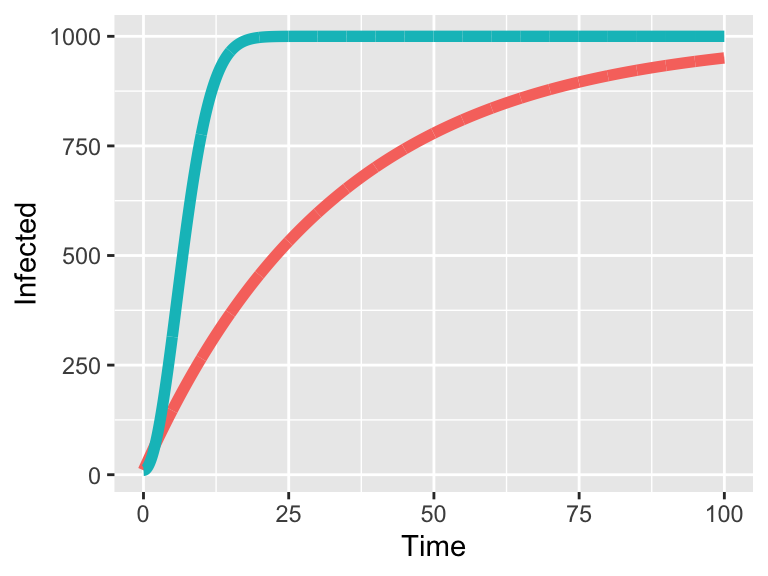

Figure 7.1: Comparison of two integrating factor solutions, Equation (7.2) in red and Equation (7.3) in blue.

Ok, let’s summarize this integrating factor approach for differential equations that can be written in the form \[\frac{dy}{dt} + f(t) \cdot y = g(t)\]

1. Calculate the integrating factor \(\displaystyle e^{\int f(t) \; dt}\). Hopefully the integral \(\displaystyle \int f(t) \; dt\) is easy to compute!
2. Next multiply the integrating factor across your equation to rewrite the differential equation as \(\displaystyle \frac{d}{dt} \left( y \cdot e^{\int f(t) \; dt} \right) = g(t) \cdot e^{\int f(t) \; dt}\).
3. Then compute the integral \(\displaystyle H(t) = \int g(t) \cdot e^{\int f(t) \; dt} \; dt\). This looks intimidating - but hopefully is manageable to compute! Don’t forget the \(+C\)!
4. Then solve for \(y(t)\): \(\displaystyle y(t) = H(t) \cdot e^{-\int f(t) \; dt} + C e^{-\int f(t) \; dt}\).

This technique is a handy way to work with equations that aren’t easily separable.