17.1 A first example

Let’s take a look at the following phase plane to this non-linear system:

\[\begin{equation} \begin{split} \frac{dx}{dt} &= y-1 \\ \frac{dy}{dt} &= x^{2}-1 \end{split} \tag{17.1} \end{equation}\]

The nullclines for this system are $y=1$ and $x=\pm1$, leading two two equilibrium solutions when we create the phaseplane:

$Phaseplane for $x'=y-1$ and $y'=x^{2}-1$.$

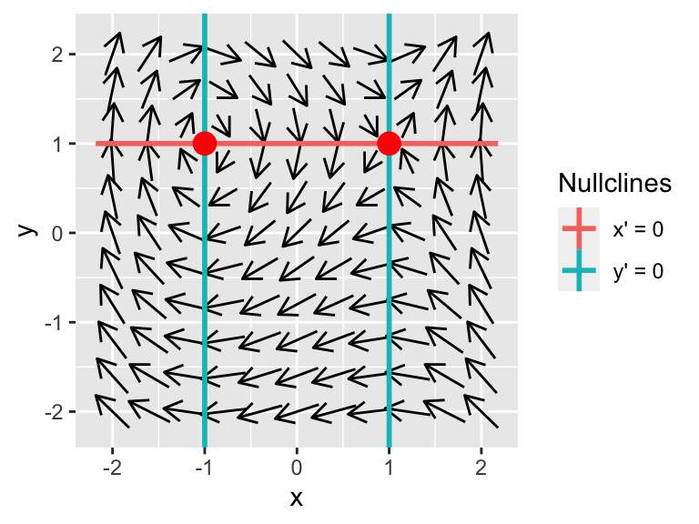
Figure 17.1: Phaseplane for $x'=y-1$ and $y'=x^{2}-1$.

From Figure 17.1, arrows on the phaseplane by the equilibrium solution at $(x,y)=(-1,1)$ seems to spiral inwards, whereas the second equilibrium solution at $(x,y)=(1,1)$ has behavior that flows in and out depending on the direction you approach. Beyond this visualization we can define additional tools to help characterize the stability of this system near the equilibrium solutions.

This section is focused on understanding the behavior near the equilibrium solutions, and in particular applying concepts of local linearization along with our understanding of linear systems. Let’s get started!