21.3 Discrete systems of equations
Finally, one way that we can extend the moose model is to account for both adult and juvenile moose populations, as with the following model:
\[\begin{equation} \begin{split} J_{t+1} &=F_{M} \cdot M_{t} \\ M_{t+1} &= G_{J} \cdot J_{t} + P_{M} \cdot M_{t} \end{split} \tag{21.2} \end{equation}\]
Equation (21.2) is a little different from (21.1) because it includes juvenile and adult moose populations, which has the following parameters:
- \(F_{M}\): represents the birth rate of new juvenile moose
- \(G_{J}\): represents the maturation rate of juvenile moose
- \(P_{M}\): represents the survival probability of adult moose
We can code up this model using R in the following way:
M0 <- 900 # Initial population of adult moose
J0 <- 100 # Initial population of juvenile moose

N <- 10 # Number of years we run the simulation
moose_two_stage <- function(f, g, p) {

  # f: birth rate of new juvenile moose
  # g: maturation rate of juvenile moose
  # p: survival probability of adult moose

  # Create a data frame of moose to return
  out_moose <- tibble(
    years = 1:N,
    adult = array(M0, dim = N),
    juvenile = array(J0, dim = N)
  )

  # And now the dynamics
  for (i in 1:(N - 1)) {
    out_moose$juvenile[i + 1] <- f * out_moose$adult[i]
    out_moose$adult[i + 1] <- g * out_moose$juvenile[i] + p * out_moose$adult[i]
  }

  return(out_moose)
}
To simulate the dynamics we just call the function moose_two_stage and plot:
moose_two_stage_rates <- moose_two_stage(
  f = 0.5,
  g = 0.6,
  p = 0.7
)

ggplot(data = moose_two_stage_rates) +
  geom_line(aes(x = years, y = adult), color = "red") +
  geom_line(aes(x = years, y = juvenile), color = "blue") +
  labs(
    x = "Years",
    y = "Moose"
  )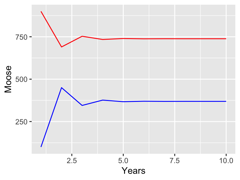
Figure 21.3: Simulation of a two stage moose population model. Adults are in red, juveniles in blue.
Looking at Figure 21.3, it seems like both populations stabilize after a few years. We could further analyze this model for stable population states (in fact, it would be similar to determining eigenvalues as in Section 18).