27.1 Meet the Fokker-Planck Equation
Let’s start with a general way to express a stochastic differential equation:
\[\begin{equation} dx = a(x,t) \; dt + b(x,t) \; dW(t) \end{equation}\]
The “solution” to this SDE will be a probability density function \(f(x,t)\). Our goal is to have a function that describes the evolution of \(f(x,t)\) in both time and space. Based on our work with birth-death processes, the probability density function \(f(x,t)\) should have the following properties:
- \(E[f(x,t)]\) is the deterministic solution to \(\displaystyle \frac{dx}{dt} = a(x,t)\).
- Var\([f(x,t)]\) is proportional to \(b(x,t)\).
We determine the probability density function through solution of the following differential equation, which is called the Fokker-Planck Equation:
\[\begin{equation} \frac{\partial f}{\partial t} = - \frac{\partial}{\partial x} \left(f(x,t) \cdot a(x,t) \right) + \frac{1}{2}\frac{\partial^{2} }{\partial x^{2}} \left(\; f(x,t) \cdot (b(x,t))^{2} \;\right) \end{equation}\]
We can write this equation in shorthand, dropping the dependence of \(x\) and \(t\) for \(f(x,t)\), \(a(x,t)\) and \(b(x,t)\): \(\displaystyle f_{t} = - (f \cdot a)_{x} + \frac{1}{2} (f \cdot b^{2})_{xx}\).
Solution. In this case \(a(x,t)=0\) and \(b(x,t)=1\), so the Fokker-Planck Equation is:
\[\begin{equation*} f_{t} = \frac{\sigma^{2}}{2} f_{xx}. \end{equation*}\]
This equation should look familiar - it is the partial differential equation for diffusion!11 The solution to this SDE is given by Equation (27.1).
\[\begin{equation} f(x,t) = \frac{1}{\sqrt{2 \pi \sigma^{2} t}} e^{-x^{2}/(2 \sigma^{2} t)} \tag{27.1} \end{equation}\]
I didn’t mention the initial condition for Equation (27.1). For this SDE the initial condition is a special function called the Dirac delta Function. We denote the Diract delta function as \(\delta(x)\). This function is a special type of probability density function, which you may study in a courses such as Functional Analysis (or Analysis). We can plot the evolution of this solution in Figure 27.1:
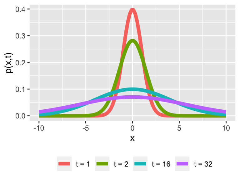
Figure 27.1: The solution to SDE \(dx = dW(t)\).
Now that we have a handle on the SDE \(dx = dW(t)\), let’s extend this next example a little more.
27.1.1 Another Fokker-Planck Equation
Consider the SDE \(dx = r \; dt + \sigma \; dW(t)\), where r and \(\sigma\) are constants. As a first step, let’s take a look at the deterministic equation: \(dx = r \; dt\). This is the differential equation \(\displaystyle \frac{dx}{dt} = r\), which has a linear function \(x(t) = rt + x_{0}\) as its solution.
We will apply the Fokker-Planck equation to characterize the solution \(f(x,t)\). In this case, the Fokker-Planck equation is
\[\begin{equation} f_{t} = -r f_{x}+ \frac{\sigma^{2}}{2} f_{xx} \tag{27.2} \end{equation}\]
Equation (27.2) is an example of a diffusion-advection equation. Amazingly this equation can be reduced to a diffusion equation through a change of variables and application of the multivariable change of variables. Let’s get to work to figure this out.
First, let \(z=x-rt\) and \(\tau = t\). This change of variables may seem odd, but our goal here is to write \(f(x,t)=f(z,\tau)\) and to develop expressions for \(f_{t}\) \(f_{x}\), and \(f_{xx}\) with this change of variables. But in order to do that, we will need to apply the multivariate chain rule (see Figure 27.2).
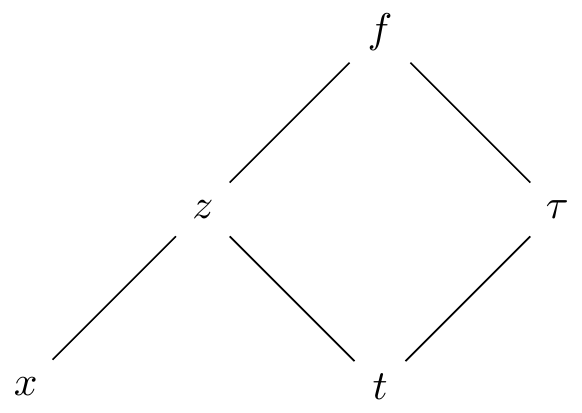
Figure 27.2: Multivariable chain rule
By the multivariable chain rule we can develop expressions for \(f_{t}\) and \(f_{x}\):
\[\begin{align*} \frac{\partial f}{\partial t} & = \frac{\partial f}{\partial \tau} \cdot \frac{ \partial \tau}{\partial t} + \frac{\partial f}{\partial z} \cdot \frac{ \partial z}{\partial t} \\ \frac{\partial f}{\partial x} & = \frac{\partial f}{\partial z} \cdot \frac{ \partial z}{\partial x} \end{align*}\]
Now let’s consider the partial derivatives \(\displaystyle \frac{ \partial \tau}{\partial t}\), \(\displaystyle \frac{ \partial z}{\partial t}\), and \(\displaystyle \frac{ \partial z}{\partial x}\).
Remember that \(z=x-r\tau\). By direct differentiation \(z_{\tau} = -r\) and \(z_{x} = 1\). Also since \(\tau=t\) then \(\tau_{t}=1\). With these substitutions, we can now re-write \(f_{t}\) and \(f_{xx}\):
\[\begin{align*} \frac{\partial f}{\partial t} & = \frac{\partial f}{\partial \tau} \cdot \frac{ \partial \tau}{\partial t} + \frac{\partial f}{\partial z} \cdot \frac{ \partial z}{\partial t} = \frac{\partial f}{\partial \tau} -r \frac{\partial f}{\partial z} \\ \frac{\partial f}{\partial x} & = \frac{\partial f}{\partial z} \rightarrow \frac{\partial^{2} f}{\partial x^{2}} = \frac{\partial^{2} f}{\partial z^{2}} \end{align*}\]
So if we re-write our original Fokker-Planck equation with the variables \(z\) and \(\tau\) we have:
\[\begin{align*} f_{t} &=-r f_{x}+ \frac{\sigma^{2}}{2} f_{xx} \\ f_{\tau} - r f_{z} &= -r f_{z} + \frac{\sigma^{2}}{2} f_{zz} \\ f_{\tau} &= \frac{\sigma^{2}}{2} f_{zz} \end{align*}\]
Ok: I’ll admit that doing change of variables may seem like it doesn’t help the situation. But guess what: with this change of variables our Fokker-Planck equation becomes a diffusion equation in the variables \(z\) and \(\tau\)! So if we can write down the solution with the variables \(z\) and \(\tau\), we can write the solution \(f(x,t)\)! Here how we do this: \(\displaystyle f(z, \tau) = \frac{1}{\sqrt{2 \pi \sigma^{2} \tau}} e^{-z^{2}/(2 \sigma^{2} \tau)}\), and then transform back into the original variables \(x\) and \(t\):
\[\begin{equation} f(x, t) = \frac{1}{\sqrt{2 \pi \sigma^{2} t}} e^{-(x-rt)^{2}/(2 \sigma^{2} t)} \end{equation}\]
Now that we have an equation, next let’s visualize the solution. Let’s take a look at some representative plots in Figure 27.3:
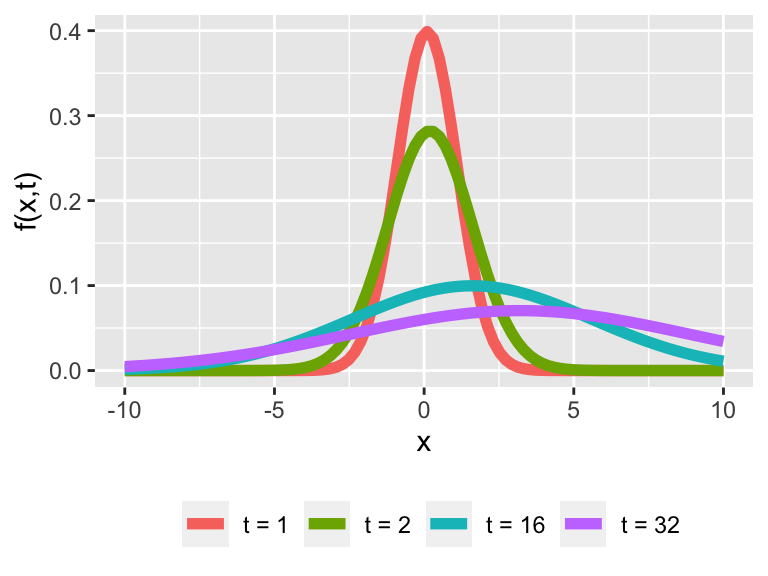
Figure 27.3: Representative plots for the solution to the SDE \(dx = r \; dt + \sigma \; dW(t)\).
Based on what we know of this distribution is that it should look like a normal distribution with mean \(\mu = rt\) and variance \(\sigma^{2} t\). What the mean and variance tells us that the mean is shifting and growing more diffuse as time increases. Remember that our solution to the deterministic equation was linear, and the mean of our distribution grows linearly as well!
Also notice in Figure 27.3 as \(t\) increases the solution shifts (“advects”) to the right. The differential equation is an example of a diffusion-advection equation, or a solution that drifts as time increases.
The examples we study here are just a few examples of how to build a deeper understanding of stochastic processes and differential equations. There is a lot of power in understanding the theoretical distribution for some test cases. Stochastic differential equations is a fascinating field of study with a lot of interesting mathematics - I hope what you learned here will make you want to study it further!
To remind you, the solution to \(p_{t} = D p_{xx}\) is \(\displaystyle p(x,t) = \frac{1}{\sqrt{4 \pi Dt} } e^{-x^{2}/(4 D t)}\). So in this case \(D = \sigma^{2}/2\).↩︎