2.6 Defining functions

We will study lots of other built-in functions for this course, but you may also be wondering how you define your own function (let’s say \(y=x^{3}\)). We need the following construct:

function_name <- function(inputs) {

  # Code

  return(outputs)
}

Here function_name serves as what you call the function, inputs are what you need in order to run the function, and outputs are what gets returned. So if we are doing \(y=x^{3}\) then we will call that function cubic:

cubic <- function(x) {
  y <- x^3
  return(y)
}

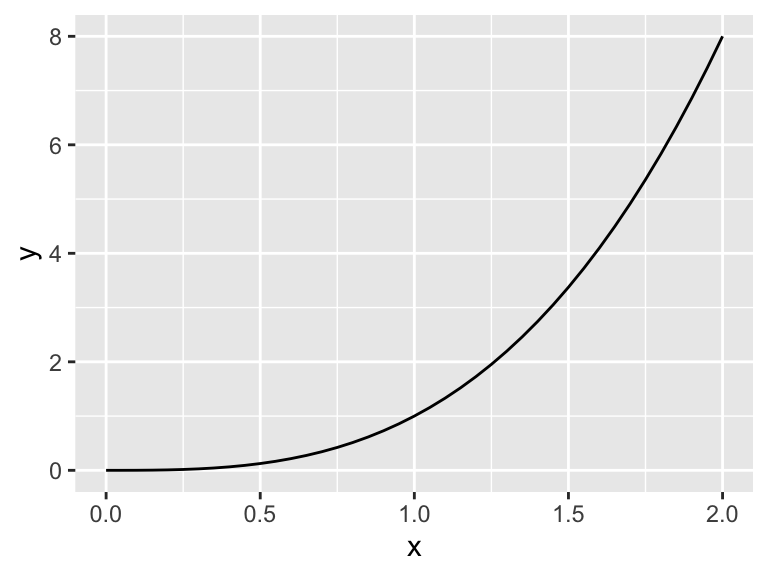
So now if we want to evaluate \(y(2)=2^{3}\) we type cubic(2). Neat! Now let’s make a plot of the graph \(y=x^{3}\) using the function defined as cubic. Here is the R code that will accomplish this:

x <- seq(from = 0, to = 2, by = 0.05)
y <- cubic(x)

my_data <- tibble(x = x, y = y)

ggplot(data = my_data) +
  geom_line(aes(x = x, y = y)) +
  labs(
    x = "x",
    y = "y"
  )

2.6.1 Functions with inputs

Sometimes you may want to define a function with different input parameters, so for example the function \(y=x^{3}+c\). To define that, we can modify the function to have input variables:

cubic_revised <- function(x, c) {
  y <- x^3 + c
  return(y)
}

So if we want to plot what happens for different values of c we have the following:

x <- seq(from = 0, to = 2, by = 0.05)


my_data_revised <- tibble(
  x = x,
  c_zero = cubic_revised(x, 0),
  c_pos1 = cubic_revised(x, 1),
  c_pos2 = cubic_revised(x, 2),
  c_neg1 = cubic_revised(x, -1)
)

ggplot(data = my_data_revised) +
  geom_line(aes(x = x, y = c_zero)) +
  geom_line(aes(x = x, y = c_pos1)) +
  geom_line(aes(x = x, y = c_pos2)) +
  geom_line(aes(x = x, y = c_neg1)) +
  labs(
    x = "x",
    y = "y"
  )

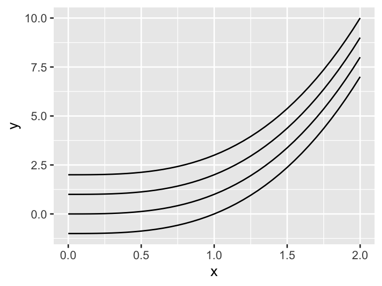
Notice how I defined multiple columns of the data frame my_data_revised in the tibble command, and then used mutiple geom_line commands to plot the data. Since we had combined the different values of c in a single data frame we didn’t need to define the data with each instance of geom_line.