9.2 Probability

In order to understand likelihood functions, first I am going to review very essential information about probability and probability distributions. Probability is the association of a set of observable events to a quantitative scale between 0 to 1. (Zero means that event is not possible, 1 means that it definitely can happen). This definition could be refined somewhat (Devore, Berk, and Carlton 2021). Events can be considered as discrete events (think counting or combinatorial problems) or continuous events. For our purposes we are only going to consider continuous events, specifically in this case the probability of a parameter obtaining a particular value.

Consider this graphic, which may be familiar to you as the normal distribution or the bell curve:

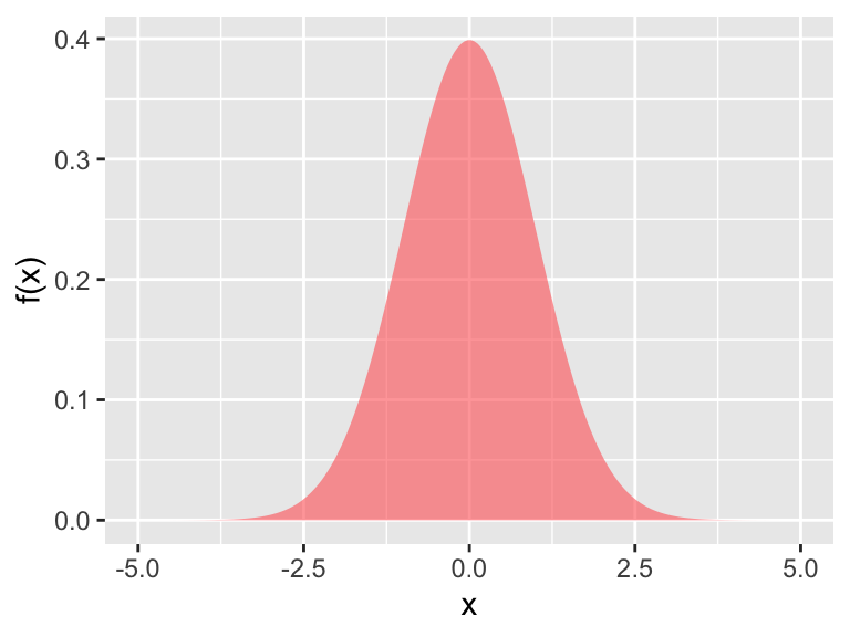
Figure 9.2: The normal distribution

We tend to think of the plot and the associated function \(f(x)\) as something with input and output (such as \(f(0)=\) 0.3989). However because it is a probability density function, the area between two points gives yields the probability of an event to fall within two values:

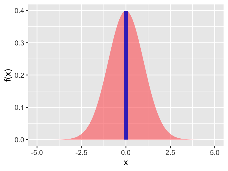
Figure 9.3: The area between two values, normally distributed

In this case, the shaded area tells us the probability that our measurement is between \(x=-0.1\) and \(x=0.1\). The value of the area, or the probability is 0.07966. When you took calculus the area was expressed as a definite integral: \(\displaystyle \int_{-0.1}^{0.1} f(x) \; dx=\) 0.07966, where \(f(x)\) is the formula for the probability density function for the normal distribution.

The basic idea is that we can assign values to an outcomes as a way of displaying our belief (confidence) in the result. With this intuition we can summarize key facts about probability density functions:

\(f(x) \geq 0\) (this means that probability density functions are positive values)
Area integrates to one (in probability, this means we have accounted for all of our outcomes)

Probability density functions also have formulas. For example, the formula for the normal distribution is \[\begin{equation} f(x)=\frac{1}{\sqrt{2 \pi} \sigma } e^{-(x-\mu)^{2}/(2 \sigma^{2})} \end{equation}\]

Where \(\mu\) is the mean and \(\sigma\) is the standard deviation

9.2.1 Other probability distributions

Beyond the normal distribution some of the more common ones we utilize in the parameter estimation are the following:

Uniform: For this distribution we must specify between a minimum value \(a\) and maximum value \(b\).

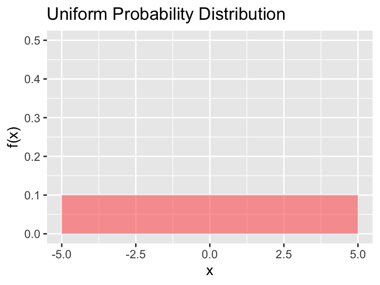
Figure 9.4: The uniform distribution

The formula for the uniform distribution is \[\begin{equation} f(x)=\frac{1}{b-a} \mbox{ for } a \leq x \leq b \end{equation}\]

Exponential: For this distribution we must specify between a rate parameter \(\lambda\).

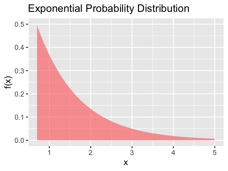
Figure 9.5: The exponential distribution

The formula for the exponential distribution is \[\begin{equation} f(x)=\lambda e^{-\lambda x} \mbox{ for } x \geq 0 \end{equation}\]

where \(\lambda\) is the rate parameter

Lognormal: This distirbution is for positive values, with mean \(\mu\) and standard deviation \(\sigma\).

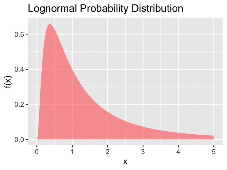
Figure 9.6: The lognormal distribution

The formula for the lognormal distribution is \[\begin{equation} f(x)=\frac{1}{\sqrt{2 \pi} \sigma x } e^{-(\ln(x)-\mu)^{2}/(2 \sigma^{2})} \mbox{ for } x \geq 0 \end{equation}\]

9.2.2 Computing and graphic probabilities in R

Here is the good news with R: the commands to generate densities and cumulative distributions are already included! There are a variety of implementations: both for the density, cumulative distribution, random number generation, and lognormal distributions from these. For the moment, the following table summarizes some common probability distributions in R.

Distribution	Key Parameters	R command	Density Example
Normal	\(\mu \rightarrow\) `mean`, \(\sigma \rightarrow\) `sd`	`norm`	`dnorm(mu=0,sd=1,seq(-5,5,length=200))`
Uniform	\(a \rightarrow\) `min`, \(b \rightarrow\) `max`	`unif`	`dunif(seq(-5,5,length=200),min = -5,max=5)`
Exponential	\(\lambda \rightarrow\) `rate`	`exp`	`dexp(seq(0,5,length=200))`
Normal	\(\mu \rightarrow\) `meanlog`, \(\sigma \rightarrow\) `sdlog`	`lnorm`	`dlnorm(seq(0,5,length=200))`

To make the graphs of these density functions in R we use the prefix d + the name (norm, exp) etc of the distribution we wish to specify, including any of the key parameters. If we don’t include any of the parameters then it will just use the defaults (which you can see by typing ?NAME where NAME is the name of the command (i.e. ?dnorm).

Example 9.1 Make a graph of the lognormal density function with \(\mu=0\) and \(\sigma=1\) from \(0 \leq x \leq 5\).

Solution. For this case we are using the defaults of the lognormal distribution. The code is the following, and plotted in Figure 9.7.

x <- seq(0, 5, length = 200)
y <- dlnorm(x) # Just use the mean defaults

# Define your data frame to plot
lognormal_data <- tibble(x, y)

ggplot() +
  geom_line(
    data = lognormal_data,
    aes(x = x, y = y)
  ) +
  labs(x = "x", y = "Lognormal density")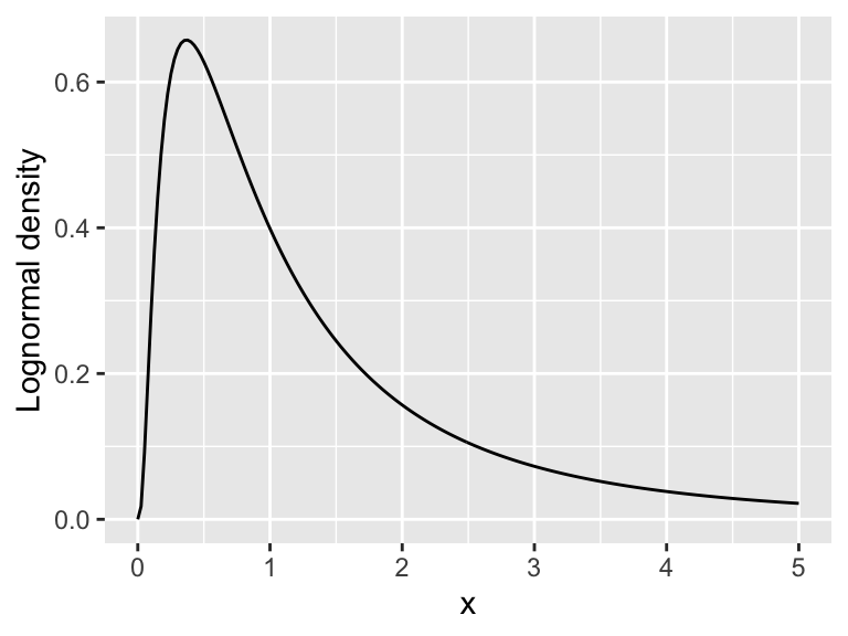

Figure 9.7: Code to plot the lognormal distribution

To determine the area between two values in a density function we use the prefix p.

Example 9.2 Use R to evaluate \(\displaystyle \int_{1}^{2} e^{-x} \; dx\).

Solution. The function \(e^{-x}\) is the exponential probability distribution with \(\lambda=1\). For this example if we wanted to find the area between two values in the exponential density in the shaded graph we would type pexp(2)-pexp(1) at the R console, which would give the value of 0.233. A visual representation of this area is shown in Figure 9.8.

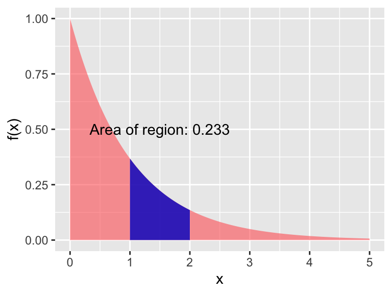
Figure 9.8: The area for the exponential distribution

References

Devore, Jay L., Kenneth N. Berk, and Matthew A. Carlton. 2021. Modern Mathematical Statistics with Applications. Third. Springer Texts in Statistics. Springer International Publishing. https://doi.org/10.1007/978-3-030-55156-8.