8.2 Fitting temperature data
Let’s take a look at a specific example. Consider the following dataset of average global temperature over time (Table 8.1:
library(tidyverse)
library(demodelr)

kable(global_temperature[1:20, ], caption = "Global Temperature from 1880")| yearSince1880 | globalTemp |
|---|---|
| 0 | 13.50 |
| 1 | 13.53 |
| 2 | 13.62 |
| 3 | 13.60 |
| 4 | 13.32 |
| 5 | 13.47 |
| 6 | 13.33 |
| 7 | 13.26 |
| 8 | 13.49 |
| 9 | 13.74 |
| 10 | 13.39 |
| 11 | 13.38 |
| 12 | 13.48 |
| 13 | 13.45 |
| 14 | 13.55 |
| 15 | 13.63 |
| 16 | 13.68 |
| 17 | 13.76 |
| 18 | 13.60 |
| 19 | 13.68 |
(This dataset can be found in the demodelr package with the name global_temperature.) To name our variables let \(Y=\mbox{ Year since 1880 }\) and \(T= \mbox{ Temperature }\). First let’s visualize the data, with time on the horizontal axis and temperature on the vertical axis:
ggplot(data = global_temperature, ) +
  geom_point(aes(x = yearSince1880, y = globalTemp),
    color = "red",
    size = 2
  ) +
  labs(x = "Y", y = "T")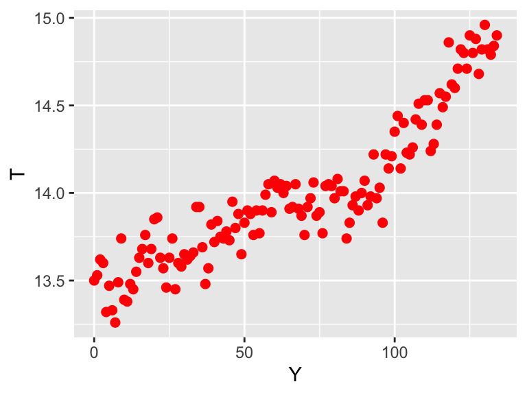
Figure 8.1: Scatterplot of global temperature data. The variable \(Y\) represents the Year since 1880 and \(T\) the temperature in degrees Celsius.
We will be working with these data to fit a function \(f(Y,\vec{\alpha})=T\). In order to fit a function in R we need three essential elements:
- We need data for the formula to interpret. This needs to be a two column data table, such as
global_temperature. - The regression formula we will use for the fit is given in the text
regressionFormula <- y ~ 1 + x. We adopt the convention that \(y\) signifies the “dependent variable” and \(x\) signifies the “independent variable,” but are named columns in a data frame. For theglobal_temperaturedataset we would write theregression_formulaasregression_formula <- globalTemp ~ 1 + yearSince1880Said differently, what this regression formula “does a linear regression where the factors are a constant term and one proportional to the independent variable.” - The command
lmstands for linear model. This is the main function that does our fitting procedure, where we need to specify the dataset we are using.
That’s it! So if we need to do a linear regression of global temperature against year since 1880 the code to do this is the following:
regression_formula <- globalTemp ~ 1 + yearSince1880

linear_fit <- lm(regression_formula, data = global_temperature)

summary(linear_fit)
##
## Call:
## lm(formula = regression_formula, data = global_temperature)
##
## Residuals:
## Min 1Q Median 3Q Max
## -0.45013 -0.11632 -0.00849 0.11326 0.36865
##
## Coefficients:
## Estimate Std. Error t value Pr(>|t|)
## (Intercept) 13.358442 0.028832 463.32 <2e-16 ***
## yearSince1880 0.009601 0.000372 25.81 <2e-16 ***
## ---
## Signif. codes: 0 '***' 0.001 '**' 0.01 '*' 0.05 '.' 0.1 ' ' 1
##
## Residual standard error: 0.1684 on 133 degrees of freedom
## Multiple R-squared: 0.8336, Adjusted R-squared: 0.8323
## F-statistic: 666.2 on 1 and 133 DF, p-value: < 2.2e-16What is printed on the console is the summary of the fit results. This summary contains several interesting things that you would study in advanced courses in statistics, but here is what we will focus on:
- The estimated coefficients (
Coefficients:) of the linear regression. The columnEstimatelists the constants in front of our regression formula \(y=a+bx\). What follows is the error on that estimate by formulas from statistics. The other additional columns concern statistical tests that show significance of the estimate. - One helpful thing to look at is the Residual standard error (
Residual standard error), which represents the overall, total effect of the differences between the model predicted values of \(\vec{y}\) and the measured values of \(\vec{y}\). The goal of linear regression is to minimize this model-data difference.
To plot the fitted equation with the regression coefficients we are going to borrow from another package called broom, which helps produce model output in what is called “tidy” data format. You can read more about broom here.
Since we are only going to use one or two functions from this package, I am going to refer to the functions I need with the syntax PACKAGE_NAME::FUNCTION.
First we will make a data frame with the predicted coefficients from our linear model:
global_temperature_model <- broom::augment(linear_fit, data = global_temperature)

glimpse(global_temperature_model)
## Rows: 135
## Columns: 8
## $ yearSince1880 <int> 0, 1, 2, 3, 4, 5, 6, 7, 8, 9, 10, 11, 12, 13, 14, 15, 16…
## $ globalTemp <dbl> 13.50, 13.53, 13.62, 13.60, 13.32, 13.47, 13.33, 13.26, …
## $ .fitted <dbl> 13.35844, 13.36804, 13.37764, 13.38725, 13.39685, 13.406…
## $ .resid <dbl> 0.141557734, 0.161956817, 0.242355900, 0.212754983, -0.0…
## $ .hat <dbl> 0.02930283, 0.02865412, 0.02801515, 0.02738595, 0.026766…
## $ .sigma <dbl> 0.1686042, 0.1684612, 0.1677079, 0.1680214, 0.1689313, 0…
## $ .cooksd <dbl> 1.098342e-02, 1.403997e-02, 3.069797e-02, 2.309589e-02, …
## $ .std.resid <dbl> 0.85304308, 0.97564433, 1.45949662, 1.28082181, -0.46247…Notice how the augment command takes the results from linear_fit with the data global_temperature. I like appending _model to the original name of the data frame to signify that there are modeled components here to work with. There is a lot to unpack with this new data frame, but the important ones are the columns yearSince1880 (the independent variable) and .fitted, which represents the fitted coefficients.
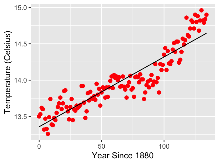
Now we are ready to graph the data along with the fitted regression line.
ggplot(data = global_temperature) +
  geom_point(aes(x = yearSince1880, y = globalTemp),
    color = "red",
    size = 2
  ) +
  geom_line(
    data = global_temperature_model,
    aes(x = yearSince1880, y = .fitted)
  ) +
  labs(
    x = "Year Since 1880",
    y = "Temperature (Celsius)"
  )