25.5 Exercises

Exercise 25.1 Consider the logistic differential equation (Equation (25.2)). In this section we set $\sigma = 1$. Re-run the code to generate one simulation with $\sigma = 0.01, \; 2, \; 10$. In each case, how does changing $\sigma$ affect the simulation run?

 

Exercise 25.2 Consider the logistic differential equation (Equation (25.2)). In this section we set $\sigma = 1$. Re-run the code to generate 100 simulations with $\sigma = 0.01, \; 2, \; 10$ and then compute the ensemble. In each case, how does changing $\sigma$ affect the ensemble average?

 

Exercise 25.3 Return back to the example of adding stochasticity to the parameter r in the logistic differential equation and the resulting spaghetti and ensemble average plots. For these plots we set $\sigma = 1$. What happens to the resulting spaghetti and ensemble plots when $\sigma = 0.01, \; 0.1, \; 10$?

 

Exercise 25.4 (Inspired by Logan and Wolesensky (2009)) Consider the logistic differential equation: $\displaystyle \frac{dx}{dt} = r x \left( 1-\frac{x}{K} \right)$. Assume there is stochasticity in the inverse carrying capacity $1/K$ (so this means you will consider $1/K + \mbox{ Noise }$).

1. Identify the deterministic and stochastic part of each of the differential equation.
2. Assume that $x(0)=3$, $r=0.8$, $K=100$, $\Delta t = 0.05$, and $\sigma=1$. Apply the Euler-Maruyama method to produce a solution, using with 200 timesteps.
3. Now do 500 simulations of this stochastic process and compare the ensemble solution.
4. Contrast your results to when we added stochasticity to the parameter $r$ in the logistic model.

 

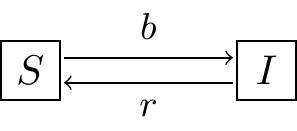
Figure 25.7: The $SIS$ model

Exercise 25.5 (Inspired by Logan and Wolesensky (2009)) An $SIS$ model is one where susceptibles $S$ become infected $I$, and then after recovering from an illness, become susceptible again. The schematic representing this is shown in Figure 25.7. While you can write this as a system of differential equations, assuming the population size is constant $N$, this simplifies to the following differential equation:

$$\begin{equation} \frac{dI}{dt} = b(N-I) I - r I \end{equation}$$

1. Determine the equilibrium solutions for this model and analyze the stability of the equilibrium solutions.
2. Assuming $N=1000$, $r=0.01$, and $b=0.005$, $I(0)=1$, apply Euler’s method to simulate this differential equation over two weeks with $\Delta t = 0.1$. Show the plot of your result.
3. Assume the transmission rate $b$ is stochastic. Write down this stochastic differential equation. Do 500 simulations of this stochastic process with $\sigma = 1$. Contrast this result to the deterministic solution.
4. Assume the recovery rate $r$ is stochastic. Write down this stochastic differential equation. Do 500 simulations of this stochastic process with $\sigma = 1$. Contrast this result to the previous results.

 

Exercise 25.6 Consider the following Lotka-Volterra (predator prey) model:

$$\begin{equation} \begin{split} \frac{dV}{dt} &= r V - kVP \\ \frac{dP}{dt} &= e k V P - dP \end{split} \end{equation}$$

1. Assume that the parameter $k$ is stochastic. Write down the stochastic differential equation, identifying the deterministic and stochastic parts to this system of equations.
   
2. Apply the Euler-Maruyama method for 100 simulations with $\sigma=0.01$ with the following values of parameters and step sizes:

• Initial condition: $V(0)=1$, $P(0)=3$
• Parameters: $r = 2$, $k = 0.5$, $e = 0.1$, and $d = 1$.
• Set $\Delta t = 0.05$ and $N=200$.

 

Exercise 25.7 Consider the following model for zombie population dynamics:

$$\begin{equation} \begin{split} \frac{dS}{dt} &=-\beta S Z - \delta S \\ \frac{dZ}{dt} &= \beta S Z + \xi R - \alpha SZ \\ \frac{dR}{dt} &= \delta S+ \alpha SZ - \xi R \end{split} \end{equation}$$

1. Let’s assume the transmission rate $\beta$ is a stochastic parameter. With this assumption, group each differential equation into two parts: terms not involving noise (the deterministic part) and terms that are multiplied by noise (the stochastic part)

• Deterministic part for $\displaystyle \frac{dS}{dt}$:
• Stochastic part for $\displaystyle \frac{dS}{dt}$:
• Deterministic part for $\displaystyle \frac{dZ}{dt}$:
• Stochastic part for $\displaystyle\frac{dZ}{dt}$:
• Deterministic part for $\displaystyle \frac{dR}{dt}$:
• Stochastic part for $\displaystyle \frac{dR}{dt}$:

2. Apply the Euler-Maruyama method to do 500 simulations of this stochastic differential equation and compute the ensemble average. For the Euler-Maruyama method apply the following values:

• $\sigma = 0.004$
• $\Delta t= 0.5$.
• Timesteps: 200.
• $\beta = 0.0095$, $\delta = 0.0001$ ,$\xi = 0.1$, $\alpha = 0.005$.
• Initial condition: $S(0)=499$, $Z(0)=1$, $R(0)=0$.

3. How does making $\beta$ stochastic affect the disease transmission? d. If we assume that the population is fixed at 500 individuals, what is interesting about your stochastic results?

References

Logan, J. David, and William Wolesensky. 2009. Mathematical Methods in Biology. 1st ed. Hoboken, N.J: Wiley.