19.1 Two dimensional linear systems: the general case

Consider the following two dimensional linear system, where \(a\), \(b\), \(c\), and \(d\) can be any number:

\[\begin{equation} \begin{pmatrix} \frac{dx}{dt} \\ \frac{dy}{dt} \end{pmatrix} = \begin{pmatrix} ax+by \\ cx+dy \end{pmatrix} = \begin{pmatrix} a & b \\ c & d \end{pmatrix} \begin{pmatrix} x \\ y \end{pmatrix} \end{equation}\]

Recall that eigenvalues are found by solving \(\displaystyle \det (A - \lambda I ) =0\), which \(\displaystyle \det (A - \lambda I )\) is computed in Equation (19.1).

\[\begin{equation} \det \begin{pmatrix} a - \lambda & b \\ c & d-\lambda \end{pmatrix} = (a-\lambda)(d-\lambda) - bc \tag{19.1} \end{equation}\]

If we multiply out Equation (19.1) we obtain the characteristic equation:

\[\begin{equation} \lambda^{2} - (a+d) \lambda + ad - bc = 0 \tag{19.2} \end{equation}\]

What is cool about Equation (19.2) is that the roots can be expressed as functions of the entries of the matrix \(A\) (\(a\), \(b\), \(c\), \(d\)). In fact, in linear algebra the term \(a+d\) is the sum of the diagonal entries, also known as the trace of a matrix. The trace of a matrix can be expressed as \(\mbox{tr}(A)\). And you may recognize that \(ad-bc\) is the same as \(\det(A)\). So our characteristic equation is can be rewritten as solving Equation (19.3):

\[\begin{equation} \lambda^{2} - \mbox{tr}(A)\lambda + \det(A)=0 \tag{19.3} \end{equation}\]

Example 19.1 Write down the characteristic equation for the system \(\vec{x}'=Ax\) where \(\displaystyle A= \begin{pmatrix} -1 & 1 \\ 0 & 3 \end{pmatrix}\) and classify the stability of the equilibrium solution.

 

Solution. We can see that \(\det(A)= -1(3) - 0(1) = -3\) and tr\((A)=2\), so our characteristic equation is \(\lambda^{2}-2\lambda -3\). If we solve \(\lambda^{2}-2\lambda -3=0\) we have \((\lambda-3)(\lambda+1)=0\), so our eigenvalues are \(\lambda=3\) and \(\lambda=-1\). Since one eigenvalue is positive and the other one is negative, the equilibrium solution is a saddle node.

Solving Equation (19.3) might be a computationally easier way to compute the eigenvalues, especially if you have a known parameter. We can also exploit this relationship even more.

Let’s say we have two eigenvalues \(\lambda_{1}\) and \(\lambda_{2}\). We make no assumptions on if they are real or imaginary or equal. But if they are eigenvalues, then they are roots of the characteristic polynomial. This means that \((\lambda-\lambda_{1})(\lambda-\lambda_{2})=0\). If we multiply out this equation we have \(\lambda^{2}-(\lambda_{1}+\lambda_{2}) \lambda + \lambda_{1} \lambda_{2}=0\). Hmmm. If we compare this equation with Equation (19.3) we have:

\[\begin{equation} \lambda^{2}-(\lambda_{1}+\lambda_{2}) \lambda + \lambda_{1} \lambda_{2} = \lambda^{2} - \mbox{tr}(A)\lambda + \det(A) \end{equation}\]

This uncovers some neat relationships - in particular tr\((A)=(\lambda_{1}+\lambda_{2})\) and \(\det(A)=\lambda_{1}+\lambda_{2}\). Why should we bother with this? Well this provides an alternative pathway to understand stability through the trace and determinant, in particular we have the following correspondence between the signs of the eigenvalues and the trace and determinant:

Sign of \(\lambda_{1}\)	Sign of \(\lambda_{2}\)	Tendency of solution	Sign of tr\((A)\)	Sign of \(\det(A)\)
Positive	Positive	Source	Positive	Positive
Negative	Negative	Sink	Negative	Positive
Positive	Negative	Saddle	?	Negative
Negative	Positive	Saddle	?	Negative

For the moment we will only consider real non-zero values of the eigenvalues - more specialized cases will occur later. But carefully at the table:

• If the determinant is negative, then the equilibrium solution is a saddle.
• If the determinant is positive and the trace is negative, then the equilibrium solution is a sink
• If the determinant and trace are both positive, then the equilibrium solution is a source.

Example 19.2 Use the trace and determinant relationships to classify the stability of the equilibrium solution for the linear system \(\vec{x}'=A\vec{x}\) where \(\displaystyle A= \begin{pmatrix} -1 & 1 \\ 0 & 3 \end{pmatrix}\).

 

Solution. We can see that \(\det(A)= -1(3) - 0(1) = -3\) and tr\((A)=2\). Since the determinant is negative, the equilibrium solution must be a saddle node.

  Knowing the relationships between the trace and determinant for a two-dimensional system of equations is a pretty quick and easy way to investigate stability of equilibrium solutions!

Another way to graphically represent the stability of solutions is with the trace-determinant plane (shown in Figure 19.1), with tr\((A)\) on the horizontal axis and det\((A)\) on the vertical axis:

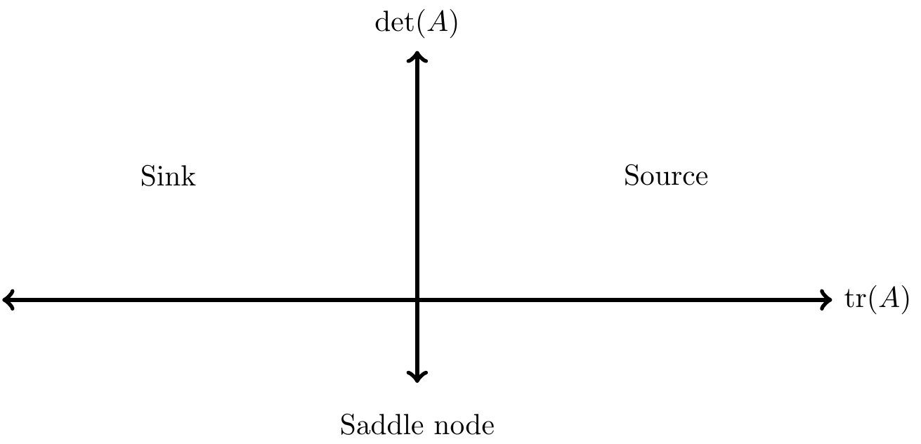
Figure 19.1: The trace-determinant plane

It also turns out that we can extend Figure 19.1 even more to include the imaginary and nonzero cases for the roots of the characteristic equation.

Firt we will apply the quadratic formula to Equation (19.3) to solve directly for the eigenvalues as a function of the trace and determinant:

\[\begin{equation} \lambda_{1,2}= \frac{\mbox{tr}(A)}{2} \pm \frac{\sqrt{ (\mbox{tr}(A))^2-4 \det(A)}}{2} \tag{19.4} \end{equation}\]

While Equation (19.4) seems like a more complicated expression, it can be shown to be consistent with our above work. Imaginary eigenvalues can be a stable or unstable spiral depending on its location in the trace-determinant plane (Figure 19.2).

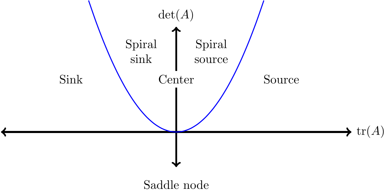
Figure 19.2: Revised trace-determinant plane.

If the discriminant (the part inside the square root for Equation (19.4), which is \((\mbox{tr}(A))^2-4 \det(A)\)) of the eigenvalue expression is negative then we have a spiral source or spiral sink depending on the positivity of the tr\((A)\).

Finally the center equilibrium occurs when the trace is exactly zero and the determinant is positive. This graphic of the trace-determinant plane is a quick way to analyze stability of a solution without a lot of algebraic analysis.