6.4 Exercises
Exercise 6.2 This problem considers the following system of differential equations: \[\begin{equation} \begin{split} \frac{dx}{dt} &= y \\ \frac{dy}{dt} &= -x \end{split} \end{equation}\]
- Determine the equations of the nullclines and equilibrium point of this system of differential equations.
- Modify the function
phaseplaneto generate a phaseplane of this system. - For each point along a nullcline, determine the resulting motion (up-down or left-right).
- Based on the work you generated, determine if the equilibrium solution is stable or unstable.
- Verify that the functions \(x(t) = \sin(t)\) and \(y=\cos(t)\) is one solution to this system of differential equations.
Exercise 6.3 Consider the following system of differential equations:
\[\begin{equation} \begin{split} \frac{dx}{dt} &= y \\ \frac{dy}{dt} &= 3x^{2}-1 \end{split} \end{equation}\]
- Determine the equations of the nullclines and equilibrium solutions for this system of differential equations.
- For each point along a nullcline, determine the resulting motion (up-down or left-right).
- Modify the function
phaseplaneto generate a phaseplane of this system. - Make a hypothesis to classify if the equilibrium point is stable or unstable.
Exercise 6.4 (Inspired by Thornley and Johnson (1990)) A plant grows propritional to its current length \(L\). Assume this proportionality constant is \(\mu\), whose rate also decreases proportional to its current value. The system of equations that models this plant growth is the following: \[\begin{equation} \begin{split} \frac{dL}{dt} &= \mu L \\ \frac{d\mu}{dt} &= -0.1 \mu \\ \end{split} \end{equation}\]
- Explain why \(L=0\) and \(\mu=0\) is the only equilibrium solution to this differential equation.
- Modify the function
phaseplaneto generate a phaseplane of this system. - Is the origin a stable equilibrium solution?
Exercise 6.5 (Inspired by Logan and Wolesensky (2009)) Red blood cells are formed from stem cells in the bone marrow. The red blood cell density \(r\) satisfies an equation of the form
\[\begin{equation} \frac{dr}{dt} = \frac{0.2r}{1+r^{2}} - 0.1 r, \end{equation}\]
- What are the equilibrium solutions for this differential equation?
- Modify the function
phaseplaneto generate a phaseline for this differential euqation for \(0 \leq t \leq 5\) and \(0 \leq r \leq 5\). - Based on the phaseline, are the equilibrium solutions stable or unstable?
Exercise 6.6 (Inspired by Hugo van den Berg (2011)) Organisms that live in a saline environment biochemically maintain the amount of salt in their blood stream. An equation that represents the level of \(S\) in the blood is the following:
\[ \frac{dS}{dt} = 1 + 0.3 \cdot (3 - S) \]
- What are the equilibrium solutions for this differential equation?
- Modify the function
phaseplaneto generate a phaseline for this differential euqation for \(0 \leq t \leq 10\) and \(0 \leq S \leq 10\). - Based on the phaseline, are the equilibrium solutions stable or unstable?
Exercise 6.7 (Inspired by Hugo van den Berg (2011)) The core body temperature (\(T\)) of a mammal is coupled to the heat production (scaled by heat capacity \(Q\)) with the following system of differential equations: \[\begin{equation} \begin{split} \frac{dT}{dt} &= Q + 0.5 \cdot (20-T) \\ \frac{dQ}{dt} &= 0.1 \cdot (38-T), \end{split} \end{equation}\]
- Determine the equations of the nullclines and equilibrium point of this system of differential equations.
- For each point along a nullcline, determine the resulting motion (up-down or left-right).
- Make a hypothesis to classify if the equilibrium point is stable or unstable.
Exercise 6.8 Consider the following system of differential equations for the lynx-hare model: \[\begin{align} \frac{dH}{dt} &= r H - b HL \\ \frac{dL}{dt} &=ebHL -dL \end{align}\]
- Determine the steady states of this system of differential equations.
- Determine equations for the nullclines, expressed as \(L\) as a function of \(H\). There should be two nullclnes for each rate.
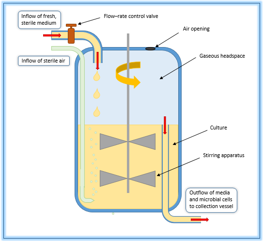
Figure 6.6: An example of a chemostat.
Exercise 6.9 (Inspired by Hugo van den Berg (2011)) A chemostat is a tank used to study microbes and ecology, where microbes grow under controlled conditions. Think of this like a large tank with nutrient-rich water being continuously cycled through, as shown in the following Figure 6.6. (Source: Wikipedia). Equations that describe the microbial biomass \(W\) and the nutrient concentration \(C\) (in the culture) are the following:
\[\begin{equation} \begin{split} \frac{dW}{dt} &= \mu W - F \frac{W}{V} \\ \frac{dC}{dt} &= D \cdot (C_{R}-C) - S \mu \frac{W}{V}, \end{split} \end{equation}\]
where we have the following parameters: \(\mu\) is the per capita reproduction rate, \(F\) is the flow rate, \(V\) is the volume of the culture solution, \(D\) is the dilution rate, \(C_{R}\) is the concentration of nutrients entering the culture, and \(S\) is a stoichiometric conversion of nutrients to biomass.
- Write the equations of the nullclines for this differential equation.
- Determine the equilibrium solutions for this system of differential equations.
- Generate a phaseplane for this differential equation with the values \(\mu=1\), \(D=1\), \(C_{R}=2\) and \(S=1\) and \(V=1\).
- Classify the stability of the equilbrium solutions.
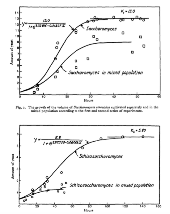
Exercise 6.10 A classical paper Experimental Studies on the Struggle for Existence: I. Mixed Population of Two Species of Yeast by Gause (1932) examined two different species of yeast growing in competition with each other. The differential equations given for two species in competition are:
\[\begin{equation} \begin{split} \frac{dy_{1}}{dt} &= -b_{1} y_{1} \frac{(K_{1}-(y_{1}+\alpha y_{2}) )}{K_{1}} \\ \frac{dy_{2}}{dt} &= -b_{2} y_{2} \frac{(K_{2}-(y_{2}+\beta y_{1}) )}{K_{2}}, \\ \end{split} \end{equation}\]
where \(y_{1}\) and \(y_{2}\) are the two species of yeast with the parameters \(b_{1}, \; b_{2}, \; K_{1}, \; K_{2}, \; \alpha, \; \beta\) describing the characteristics of the yeast species.
- Determine the equilibrium solutions for this differential equation. Express your answer in terms of the parameters \(b_{1}, \; b_{2}, \; K_{1}, \; K_{2}, \; \alpha, \; \beta\).
- Gause computed the following values of the parameters: \(b_{1}=0.21827, \; b_{2}=0.06069, \; K_{1}=13.0, \; K_{2}=5.8, \; \alpha=3.15, \; \beta=0.439\). Using these values, what would be the predicted values for the equilibrium solutions?
- Use the function
systemsto solve this system of differential equations numerically. - Figure 6.7 is from Gause (1932) and shows the experimental population values ``in mixed population’’. Use the graph to estimate the equilibrium solutions for both species. How close (or how far from) the equilibrium solutions are Gause’s results to your computed equilibrium solutions?