20.3 Limit Cycles and Bifurcations with systems of equations

The previous examples we have studied examine the stability of an equilibrium solution as a parameter changes. An extension of an equilibrium solution (as a point in space) is an equilibrium solution that is a function.

Consider the following highly nonlinear system: \[\begin{equation} \begin{split} \frac{dx}{dt} =-y-x(x^2+y^2-1) \\ \frac{dy}{dt}=x-y(x^2+y^2-1) \end{split} \tag{20.2} \end{equation}\]

The phase plane for Equation (20.2) is shown in Figure 20.7. You can verify that Equation (20.2) system has an equilibrium solution at the point $x=0$, $y=0$.

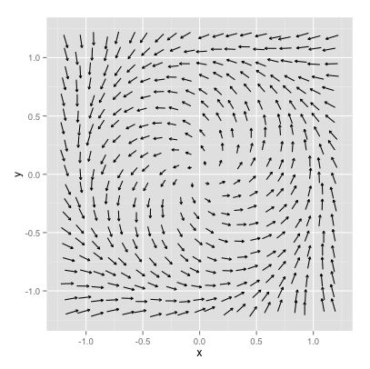
$Phase plane for Equation \ref(eq:limit-cycle-20)$

Figure 20.7: Phase plane for Equation (eq:limit-cycle-20)

However the phase plane suggests there might be other equilibrium solutions. To further explore this, let’s look at the phase plane with some solution curves in Figure 20.8:

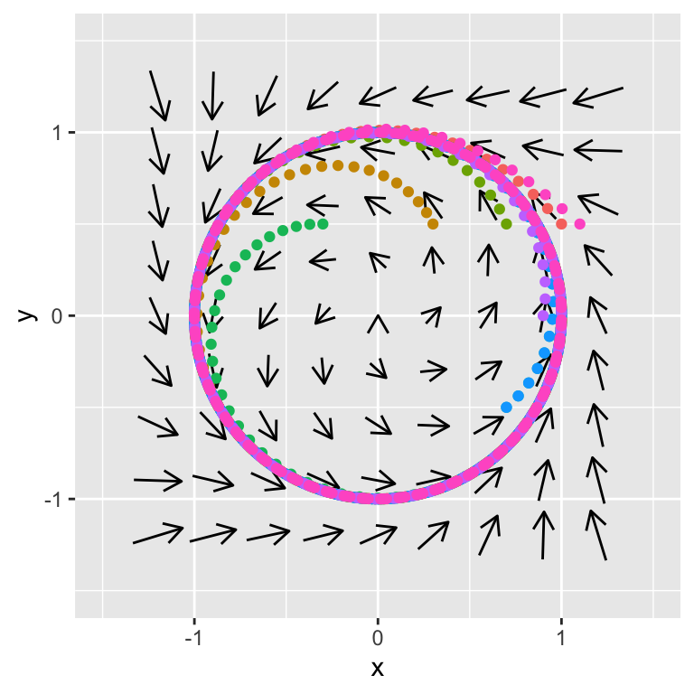
$Phase plane with solutions curves for Equation \@ref(eq:limit-cycle-20)$

Figure 20.8: Phase plane with solutions curves for Equation (20.2)

What is interesting in Figure 20.8 that the solution is tending towards a circle of radius 1 (or the equation $x^{2}+y^{2}=1$). This is an example of an equilibrium solution that is a curve rather than a specific point. We can transform this system from $x$ and $y$ to a single new variables $X$ (see Exercise 20.6).

\[\begin{equation} \frac{dX}{dt} = -X(X-1), \mbox{ where } X=r^{2}. \tag{20.3} \end{equation}\]

How Equation (20.2) transforms to Equation (20.3) is by applying a polar coordinate transformation to this system. By applying stability analysis for Equation (20.3) we can show that the equilibrium solution $X=0$ is unstable (meaning the origin $x=0$ and $y=0$ is an unstable solution) and the circle of radius 1 is stable (which is the equation $x^{2}+y^{2}=1$). In this case we would say $r=1$ is a stable limit cycle. You will study a similar system in Exercises 20.6 and 20.7.

Equation (20.3) is an example of next steps with studying the qualitative analysis of systems. While we have focused on bifurcation of equilibrium solutions, hopefully this brief introduction will pique your interest in further study of bifurcations.

The most important part in studying bifurcations is analyzing examples. I’ve provided a lot of exercises where you will construct bifurcation diagrams for one and two-dimensional equations. Given an equation with a parameter, it is helpful to construct some sample phaselines / phaseplanes before analyzing stability in general using the stability test or the trace-determinant plane.