10.3 Extending the cost function

The cost function \(S(b)\) can be extended additionally to incorporate other types of data. For example, if we knew there was a given range of values that would make sense (say \(b\) is near 1.3 with a standard deviation of 0.1), we should be able to incorporate this information into the cost function. A naive approach would be just to add in some additional squared term (\(\tilde{S}(b)\), Equation (10.4)), which is plotted in Figure 10.3.

\[\begin{equation} \tilde{S}(b)=(3-b)^2+(5-2b)^2+(4-4b)^2+(10-4b)^2 + \frac{(b-1.3)^2}{0.1^2} \tag{10.4} \end{equation}\]

## Warning: Removed 191 row(s) containing missing values (geom_path).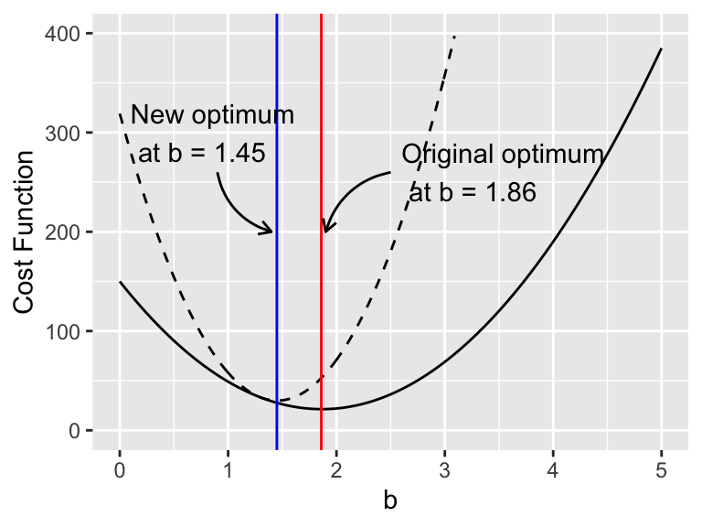

Figure 10.3: Comparing two cost functions \(S(b)\) (black) and \(\tilde{S}(b)\) (black dashed line)

Aha! Figure 10.3 shows how the revised cost function \(\tilde{S}(b)\) changes the optimum value. Numerically this works out to be \(\tilde{b}=\) 1.45. In a homework problem you verify this new minimum value and compare the fitted value to the value of \(b=1.86\).

Adding this prior information seems like an effective approach - and perhaps is applicable for problems in the sciences. Many times a scientific study wants to build upon the existing body of literature and to take that into account. This approach of including prior information into the cost function borrows elements of Bayes’ rule - so let’s have a digression into what that means.