5.2 Phase lines for differential equations
While it is one thing to determine where the equilibrium solutions are, we are also interested in classifying the stability of the equilibrium solutions. To do this investigate the behavior of the differential equation around the equilibrium solutions, using facts from calculus:
- If \(\displaystyle \frac{dy}{dt}<0\), the solution \(y(t)\) is decreasing.
- If \(\displaystyle \frac{dy}{dt}>0\), the solution \(y(t)\) is increasing.
Let’s apply this logic to our differential equation \(\displaystyle \frac{dy}{dt}=- y\). We know that if \(y=3\), \(\displaystyle \frac{dy}{dt}=- 3 <0\), so we say the function is decreasing to \(y=0\). If \(y=-2\), \(\displaystyle \frac{dy}{dt}=- (-2) = 2 >0\), so we say the function is increasing to \(y=0\). This can be represented neatly in the phase line diagram for Figure 5.3:

Figure 5.3: Phase line to \(y'=-y\).
Because the solution is increasing to \(y=0\) when \(y <0\), and decreasing to \(y=0\) when \(y >0\), we say that the equilibrium solution is stable, which is also confirmed by the solutions we plotted above.
Solution. In this case the equilibrium solution is still \(y=0\). We will need to consider three different cases for the stability depending on the value of \(k\) (\(k>0\), \(k<0\), and \(k=0\)):
- When \(k<0\), the phase line will be similar Figure 5.3.
- When \(k>0\) the phase line will be is shown in the Figure 5.4. We say in this case that the equilibrium solution is unstable, as all solutions flow away from the equilibrium. Several different solutions are shown in Figure 5.5
- When \(k=0\) we have the differential equation \(\displaystyle \frac{dy}{dt}=0\), which has \(y=C\) as a general solution. For this special case the equilibrium solution is neither stable or unstable3.
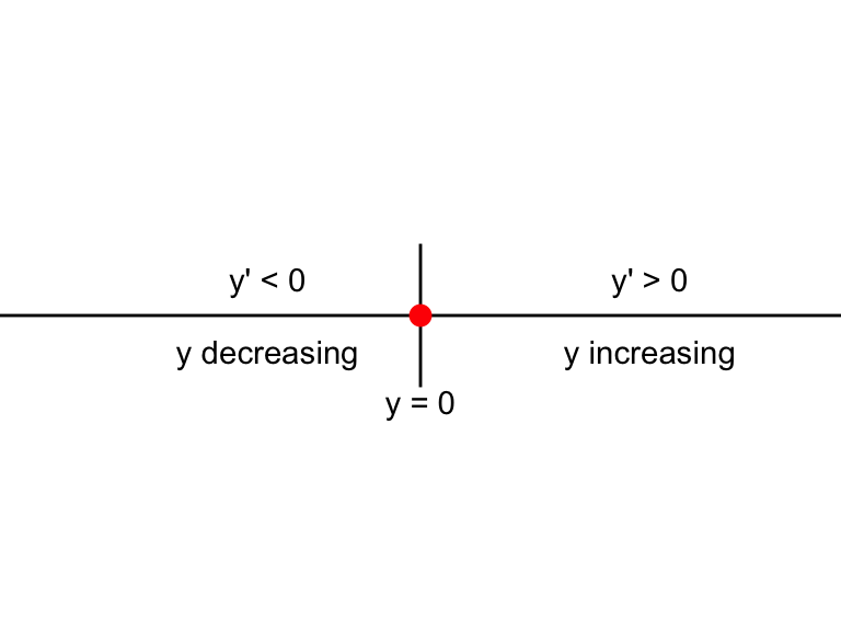
Figure 5.4: Phaseline for \(y'=ky\), with \(k>0\).
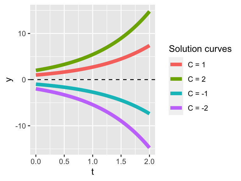
Figure 5.5: Solution curves for \(y'=ky\), with \(k>0\).
Solution. This differential equation has equilbrium solutions when \(N(1-N)=0\), or \(N=0\) or \(N=1\). We evaluate the stability of the solutions in the following table:
| Test point | Sign of \(N'\) | Tendency of solution |
|---|---|---|
| \(N=-1\) | Negative | Decreasing |
| \(N=0\) | Zero | Equilibrium solution |
| \(N=0.5\) | Positive | Increasing |
| \(N=1\) | Zero | Equilibrium solution |
| \(N=2\) | Negative | Decreasing |
Notice how the selected test points in the first column are either the the left or the right of the equilbrium solution. We can also represent the information in the table using a phase line diagram (Figure 5.6), but in this case we need to include two equilibrium solutions.
The table and Figure 5.6 confirms that \(N\) is moving away from \(N=0\) (either decreasing when \(N\) is less than 0 and increasing when \(N\) is greater than 0) and moving towards \(N=1\) (either increasing when \(N\) is between 0 and 1 and decreasing when \(N\) is greater than one.
These results suggest that equilibrium solution at \(N=0\) to be unstable and at \(N=1\) to be stable.
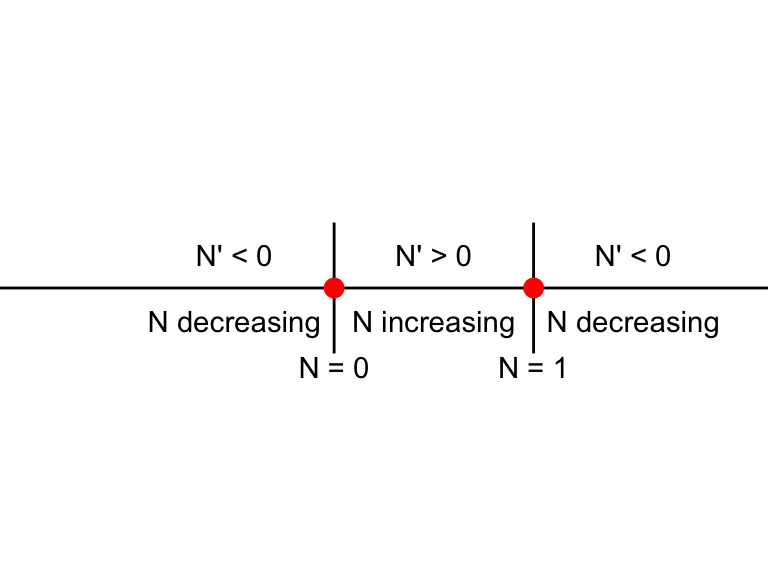
Figure 5.6: Phase line diagram for the differential equation \(N'=N(1-N)\).
Other than writing the words in the phase line diagram, we also use arrows to signify increasing or decreasing in the solutions.