14.1 Why bother with more models?
Recall the key problem of parameter estimation, which can be generally stated as the following:
Determine the set of parameters \(\vec{\alpha}\) that minimize the difference between data \(\vec{y}\) and the output of the function \(f(\vec{x}, \vec{\alpha})\) and measured error \(\vec{\sigma}\).
Let’s say we have not just one model \(f(\vec{x}, \vec{\alpha})\), but an alternative model for the data \(\vec{y}\) that can be represented as \(g(\vec{x}, \vec{\beta})\). Between these two models (\(f\) and \(g\)), how would we determine which one is “best?”
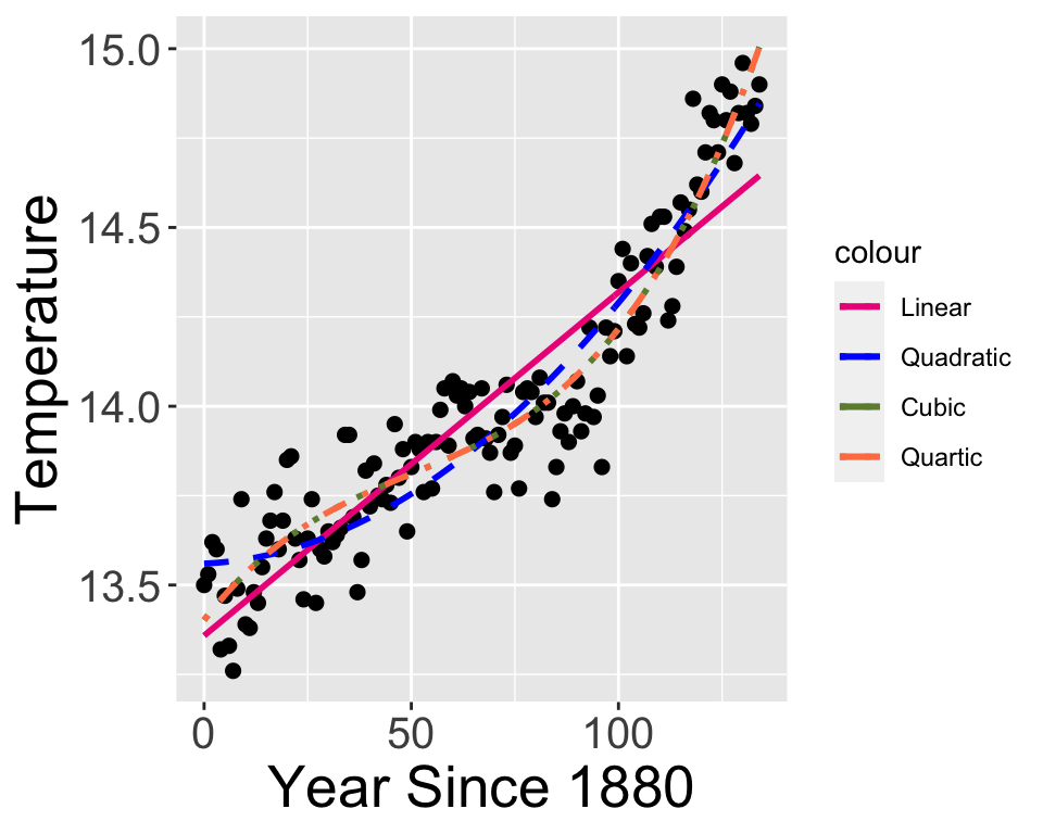
Let’s talk about a specific example. Let’s focus on the dataset global_temperature in the demodelr library. This dataset represents the average global temperature determined by NASA using local temperature data. When we did linear regression on the global temperature dataset the quadratic and cubic models were approximately the same (Figure 14.1):

Figure 14.1: Comparison of global temperature data with various polynomial fitted models.
The variation in the different models fits for Figure 14.1 shows how different, but similar, the model results can be depending on the choice of regression function. In some cases, the Log likelihood decreases (indicating a more likely model), with a smaller root mean square error (RMSE, indicating the fitted model more closely matches the observations).
| Model | Log Likelihood | RMSE |
|---|---|---|
| Linear | 49.917 | 0.167 |
| Quadratic | 74.385 | 0.139 |
| Cubic | 89.49 | 0.125 |
| Quartic | 89.599 | 0.125 |
Further model evaluation can be examined by the following:
- Compare the measured values of \(\vec{y}\) to the modeled values of \(\vec{y}\) in a 1:1 plot. Does \(g\) does a better job predicting \(\vec{y}\) than \(f\)?
- Related to that, compare the likelihood function values of \(f\) and \(g\). We would favor the model that has the lower log likelihood.
- Compare the number of parameters in each model \(f\) and \(g\). We would favor the model that has the fewest number of parameters.