9.1 Linear regression, part 2

Assume we have the following (limited) number of points where we wish to fit a function of the form \(y=bx\).

x	y
1	3
2	5
4	4
4	10

For this example we are forcing the intercept term \(a\) to equal zero - for most cases you will just fit the linear equation (see Exercise 9.7 where you will consider the intercept \(a\)). Figure 9.1 displays a quick scatterplot of these data:

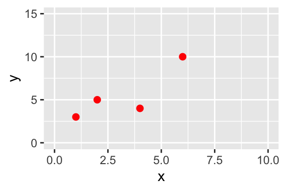
Figure 9.1: A scatterplot of a small dataset.

The goal here is to work to determine the value of \(b\) that is most likely (in other words, consistent) with the data. However, before we tackle this further we need to understand how to quantify more likely in a mathematical sense. In order to do this, we need to take a quick excursion into probability distributions. Let’s go!