4.1 Defining an Algorithm
Here would be an algorithm that would describe our process to determine a solution to a differential equation:
- Determine the locally linear approximation at a given point.
- Forecast out to another time value.
- Repeat the locally linear approximation.
If we continue on in this way, let’s take a look at how our approximation would do after several days:
| \(t\) | Approximate Solution | Actual Solution |
|---|---|---|
| 90 | 118.4 | 117 |
| 95 | 119.9 | 118.6 |
Now it seems that our approximation isn’t so accurate as time goes on. What if we updated the infection rate every half day? I know this means that we would be doing additional work (more iterations), but taking smaller timesteps goes hand in hand with more accurate solutions. Let’s start out smaller with the first few timesteps:
| \(t\) | \(I\) | \(\displaystyle \frac{dI}{dt}\) | \(\displaystyle \frac{dI}{dt} \cdot \Delta t\) |
|---|---|---|---|
| 0 | 10 | 3 | 1.5 |
| 0.5 | = 10 + 1.5 = 11.5 | 2.96 | 1.48 |
| 1 | = 11.5 + 1.48 = 12.98 | 2.92 | 1.46 |
| 1.5 | = 12.92 + 1.46 = 14.38 | 2.88 | 1.44 |
| 2 | = 14.38 + 1.44 = 15.82 |
Notice how we have started to build up a way to organize how to compute the solution. Each column is a “step” of the method, computing the solution at a new timestep based on our step size \(\Delta t\). The third column just computes the value of the derivative for a particular time and \(I\), and then the fourth column is the increment size, or the amount we are forecasting the solution will grow by to the next timestep. (There are other ways to think about this, but if you have a rate of change multiplied by a time increment this will give you an approximation to the net change in a function.)
This idea of approximate, forecast, repeat is the heart of many numerical methods that approximate solutions to differential equations. The particular method that we have developed here is called Euler’s Method. We display the results from additional steps in Figure 4.1.
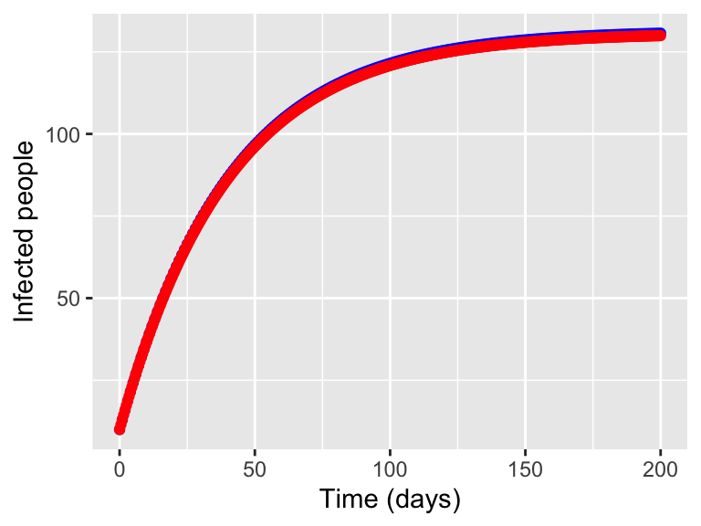
Figure 4.1: Approximation of a solution using local linearity
You may notice that the approximation in Figure 4.1 compares very favorably to the actual solution function. At the end, we have the following comparisons:
| \(t\) | Euler’s Method (\(\Delta t = 1\)) | Euler’s Method (\(\Delta t = 0.5\)) | Actual Solution |
|---|---|---|---|
| 190 | 130.5 | 129.7 | 129 |
| 195 | 130.6 | 129.8 | 129.1 |
| 200 | 130.7 | 129.9 | 129.2 |
There is a tradeoff here - the smaller stepsizes you have the more work it will take to compute you solution. You may have seen a similar tradeoff in Calculus when you explored numerical integration and Riemann sums.