17.7 Exercises
Exercise 17.1 Consider the following nonlinear system:
\[\begin{equation} \begin{split} \frac{dx}{dt} &= y-1 \\ \frac{dy}{dt} &= x^{2}-1 \end{split} \end{equation}\]
- Verify that this system has equilibrium solutions at \((-1,1)\) and \((1,1)\).
- Construct the Jacobian matrix at the equilibrium solutions at \((-1,1)\) and \((1,1)\).
- With the Jacobian matrix, visualize a phaseplane at these equilbrium solutions to determine stability.
Exercise 17.2 By solving directly, show that \((H,L)=(0,0)\) and \((4,3)\) are equilibrium solutions to the following system of equations:
\[\begin{equation} \begin{split} \frac{dH}{dt} &= .3 H - .1 HL \\ \frac{dL}{dt} &=.05HL -.2L \end{split} \end{equation}\]
Exercise 17.3 Consider the following nonlinear system:
\[\begin{equation} \begin{split} \frac{dx}{dt} &= x-y \\ \frac{dy}{dt} &=-y + \frac{5x^2}{4+x^{2}}, \end{split} \end{equation}\]
- Verify that the point \((x,y)=(1,1)\) is an equilibrium solution.
- Construct the Jacobian matrix at this equilibrium solution.
- With the Jacobian matrix, visualize a phaseplane at that equilbrium solution to determine stability.
Exercise 17.4 Consider the nonlinear system
\[\begin{equation} \begin{split} \frac{dx}{dt} &= 2x+3y+xy \\ \frac{dy}{dt} &= -x + y - 2xy^{3}, \end{split} \end{equation}\]
- Verify that the point \((0,0)\) is an equilibrium solution.
- Determine the Jacobian matrix at this equilbrium solution.
- With the Jacobian matrix, visualize a phaseplane at that equilbrium solution to determine stability.
Exercise 17.5 Consider the following system:
\[\begin{equation} \begin{split} \frac{dx}{dt} &= y^{2} \\ \frac{dy}{dt} &= -\frac{2}{3} x, \end{split} \end{equation}\]
- Determine the equilibrium solution.
- Construct the Jacobian at the equilibrium solution.
- With the Jacobian matrix, visualize a phaseplane at that equilbrium solution to determine stability.
- Use the fact that that \(\displaystyle \frac{dy}{dx} / \frac{dy}{dt} = \frac{dy}{dx}\), which should yield a separable differential equation that will allow you to solve \(y(x)\). How does that solved differential equation compare to what you found by analyzing the Jacobian matrix?
Exercise 17.6 Consider the lynx-hare system with parameters \(r\), \(b\), \(e\), and \(d\):
\[\begin{equation} \begin{split} \frac{dH}{dt} &= r H - b HL \\ \frac{dL}{dt} &=ebHL -dL \end{split} \end{equation}\]
- Verify that the point \(\displaystyle \left( \frac{d}{eb}, \frac{r}{b} \right)\) is an equilibrium solution.
- Construct the Jacobian at the equilibrium solution. (Your final answer will include the parameters.)
Exercise 17.7 This problem revisits the modified lynx-hare system:
\[\begin{equation} \begin{split} \frac{dH}{dt} &= r H \left( 1- \frac{H}{K} \right) - b HL \\ \frac{dL}{dt} &=ebHL -dL \end{split} \end{equation}\]
- Verify that by rescaling of this system \(\displaystyle x=\frac{H}{K}\), \(\displaystyle y=\frac{L}{r/b}\) and \(T = r t\) we can rewrite this system as: \[\begin{equation} \begin{split} \frac{dx}{d T} &= x(1-x) - xy \\ \frac{dy}{d T} &=\frac{ebK}{r}xy -\frac{d}{r}y \end{split} \end{equation}\]
- Determine the three equilibrium solutions of this rescaled system.
- Evaluate the Jacobian at each of the equilibrium solutions.
- With your Jacobian, select reasonable values of the parameters to generate a phaseplane diagram and classify the stability of each equilibrium solution.
- How does this revised system compare to the stability of the regular lynx-hare model?
Exercise 17.8 (Inspired by Logan and Wolesensky (2009)) A model for the spread of a disease where people recover is given by the following differential equation:
\[\begin{equation} \begin{split} \frac{dS}{dt} &= -\alpha SI \\ \frac{dI}{dt} &= \alpha SI - \gamma I \\ \frac{dR}{dt} &= \gamma I, \end{split} \end{equation}\]
- Determine the equilibrium solutions for this system of equations.
- Construct the Jacobian for each of the equilibrium solutions.
- Let \(\alpha=0.001\) and \(\gamma = 0.2\). With the Jacobian matrix, generate the phase plane (using the equations for \(\displaystyle \frac{dS}{dt}\) and \(\displaystyle \frac{dI}{dt}\) only) for all of the equilibrium solutions and classify their stability.
Exercise 17.9 (Inspired by Logan and Wolesensky (2009)) A population of fish used as food is an example of a renewable resource. This population decreases due to harvesting the fish. As long as the rate of harvest is smaller than the replacement rate, theoretically the population would be considered a renewable resource. However fish do have natural predators, which may also be harvested at the same time. A model that describes this interaction is
\[\begin{equation} \begin{split} \frac{dN}{dt} &= rN - cNP - \rho E N \\ \frac{dP}{dt} &= bcNP - mP - \sigma EP, \end{split} \end{equation}\]
where \(E\) is the fishing effort and \(\rho\) and \(\sigma\) are the catchability coefficients for the prey and predator.
- Determine all the equilibrium solutions for this model.
- Construct the Jacobian matrix for each of the the equilibrium solutions.
- Select different parameter values. With the Jacobian, construct a phase plane diagram for each of the equilibrium solutions.
- In the absence of fishing \(E=0\). How do these equilibrium solutions compare to the ones from the previous part?
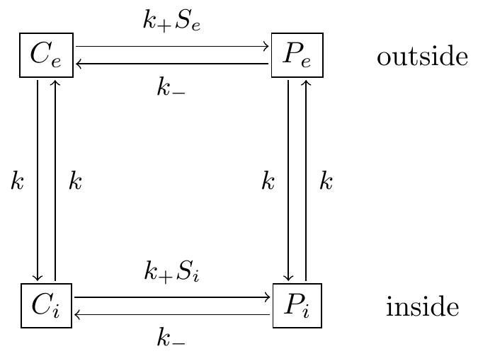
Figure 17.3: Glucose transporter reaction schemes.
Exercise 17.10 (Inspired by Keener et al. (2009)) The chemical glucose is transported across the cell membrane using a carrier proteins. These proteins can have different states (open or closed) that can be bound to a glucose substrate. The schematic for this reaction is shown in Figure 17.3. The system of differential equations describing this reaction is:
\[\begin{equation} \begin{split} \frac{dp_{i}}{dt} &= k p_{e} - k p_{i} + k_{+} s_{i}c_{i}-k_{i}p_{i} \\ \frac{dp_{e}}{dt} &= k p_{i} - k p_{e} + k_{+} s_{e}c_{e}-k_{-}p_{e} \\ \frac{dc_{i}}{dt} &= k c_{e} - k c_{i} + k_{-} p_{i}-k_{+}s_{i}c_{i} \\ \frac{dc_{e}}{dt} &= k c_{i} - k c_{e} + k_{-} p_{e}-k_{+}s_{e}c_{e} \end{split} \end{equation}\]
- We can reduce this to a system of three equations. First show that \(\displaystyle \frac{dp_{i}}{dt} + \frac{dp_{e}}{dt}+ \frac{dc_{i}}{dt} + \frac{dc_{e}}{dt} = 0\). Given that \(p_{i}+p_{e}+c_{i}+c_{e}=C_{0}\), where \(C_{0}\) is constant, use this equation to eliminate \(p_{i}\) and write down a system of three equations.
- Determine the equilibrium solutions for this new system of three equations.
- Construct the Jacobian matrix for each of these equilibrium solutions.