1.2 Modeling in context: the spread of a disease
Consider the data in Figure 1.1, which come from an Ebola outbreak in Sierra Leone in 2014. Ebola is a fatal disease so we can also consider the vertical axis in Figure 1.1 to represent total infections due to Ebola.
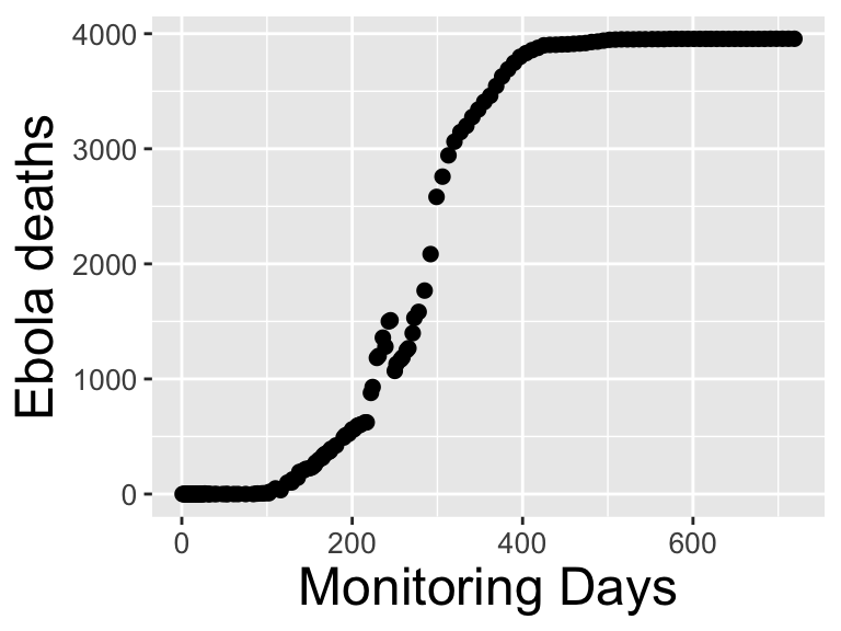
Figure 1.1: An Ebola outbreak in Sierra Leone
Constructing a model from disease dynamics is part of the field of mathematical epidemiology. How we construct a mathematical model of the spread of this outbreak largely depends on the assumptions underlying the dynamics of the disease, such as considering the rate of spread of Ebola. For our purposes here we focus on the population level (person to person) spread of Ebola. Other types of models could focus on the immune response in a single person - perhaps with a goal to design effective types of treatments to reduce the severity of infection.
Here are three initial assumptions one can make regarding the spread of Ebola:
- The infection rate is proportional to the number of people infected.
- The infection rate is proportional to the number of people not infected.
- The infection rate is proportional to the number of infected people coming into contact with those not infected.
Let’s see what each of these mathematical models would look like if we wrote down a mathematical equation. Since we are discussing rates of infection, this means we will need a rate of change or derivative. Let’s use the letter \(I\) to represent the number of people that are infected.
1.2.1 Model 1: Infection rate proportional to number infected.
The first assumption states that the infection rate is proportional to the number of people infected. Translated into an equation this would be the following:
\[\begin{equation} \frac{dI}{dt} = kI \tag{1.1} \end{equation}\]
In Equation (1.1) \(k\) can be thought of as a proportionality constant, with units of time\(^{-1}\) for consistency. Equation (1.1) is an example of a differential equation, which is just a mathematical equation with rates of change.
The solution to a differential equation is a function \(I(t)\).1 When we ``solve’’ a differential equation we determine the family of functions consistent with our rate equation. There are a lot of techniques we can use to do that, and we will examine a few later.
Back to this proportionality constant \(k\) - another term for it is a parameter. We can always try to solve an equation without specifying the parameter - and then if we wanted to plot a solution the parameter would also be specified. In some situations we may not be as concerned with the particular value of the parameter but rather its influence on the long-term behavior of the system (this is one aspect of bifurcation theory). Otherwise we can use the collected data shown above with the given model to determine the value for \(k\). This combination of a mathematical model with data is called data assimilation or model-data fusion.
Before we think about possible solutions to our differential equation, let’s try to reason if the first model would be plausible. The first model assumptions states that the rate of change (the amount of increase) gets larger with the more sick people there are. While this may seem reasonable initially, it could grows quickly unreasonable when the pandemic spreads. In the case of Ebola or any other infectious disease, stringent public health measures would be enacted if the number of people infected become too large2. Following public health measures we would expect that the rate of infection would decrease and the number of deaths to slow. So perhaps the second model might be a little more plausible. At some point the number of people who are not sick will reach zero, making the rate of infection be zero (or no increase).
1.2.2 Model 2: Infection rate proportional to number NOT infected.
In this description notice how we are talking about people who are sick (which we have denoted as \(I\)) and people who are not sick. This looks like we might need to introduce another variable for the ``not sick" people, which we will call \(S\), or susceptible. So the differential equation we would write down would be:
\[\begin{equation} \frac{dI}{dt} = kS \tag{1.2} \end{equation}\]
We are still using the parameter \(k\) as with the previous model. Also note we introduced the second variable \(S\) is in Equation (1.2). Because we have introduced another variable \(S\) we should also include a differential equation for how \(S\) changes as well. One way that we can do this is by considering our entire population as consisting of two groups of people: \(S\) and \(I\). Infection brings someone over from \(S\) to \(I\), which we have in Figure 1.2:
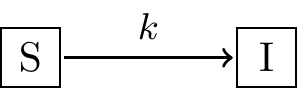
Figure 1.2: Schematic diagram for Model 1
There are three reasons why I like to use diagrams like Figure 1.2: (1) they help organize my thinking about a mathematical model (2) any assumed parameters (\(k\)) are listed, and (3) they help me to see that rates can be conserved. If I enter into the box for \(I\), then someone is leaving \(S\). So then the rate of change equation for \(S\) is \(\displaystyle \frac{dS}{dt} = -kS\). Together with the differentail equation for \(I\) I have the following:
\[\begin{equation} \begin{split} \frac{dS}{dt} &= -kS \\ \frac{dI}{dt} &= kS \end{split} \tag{1.3} \end{equation}\]
Equation (1.3) is an example of a coupled differential equation. In order to ``solve" the system we need to determine functions for \(S\) and \(I\). This coupled set of equations looks a little clunky, but there is something interest going on if we add the rates \(\displaystyle \frac{dS}{dt}\) and \(\displaystyle \frac{dI}{dt}\) together. Algebraically we have:
\[\begin{equation} \frac{dS}{dt} + \frac{dI}{dt} = \frac{d(S+I)}{dt} = 0 \tag{1.4} \end{equation}\]
Recall from calculus that if a rate of change equals zero then the function is constant. In this case, the variable \(S+I\) is constant, or we can also call \(S+I=N\), the number of people in the population. This means that \(S=N-I\), so we can re-write Equation (1.3) with a single equation:
\[\begin{equation} \frac{dI}{dt} = k(N-I) \tag{1.5} \end{equation}\]
This second model does have some limiting behavior to this model as well. As the number of infected people reaches \(N\) (the total population size), the values of \(\displaystyle \frac{dI}{dt}\) approaches zero, meaning \(I\) doesn’t change. There is one caveat to this - if there are no infected people around (\(I=0\)) the disease can still be transmitted, which might make not good biological sense.
1.2.3 Model 3: Infection rate proportional to infected meeting not infected.
The third model rectifies some of the shortcomings of the second model (which rectified the shortcomings of the first model). The third model states that the rate of infection is due to those who are sick infecting those who are not sick. This would sort of scenario would also make some sense, as it focuses on the transmission of the disease between susceptibles and infected people. So if nobody is sick (\(I=0\)) then the disease is not spread. Likewise if there are no susceptibles (\(S=0\)), the disease is not spread as well.
In this case the diagram outlining the third model looks something like this:
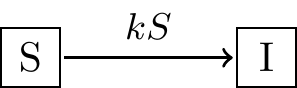
Figure 1.3: Schematic diagram for Model 3
Notice how in Figure 1.3 there is an additional \(S\) associated with \(k\) to show how the rate of infection depends on \(S\). The differential equations that describe the scenario outlined in Figure 1.3 are the following:
\[\begin{align*} \frac{dS}{dt} &= -kSI \\ \frac{dI}{dt} &= kSI \end{align*}\]
Just like before for Model 2 we can combine the two equations to yield a single differential equation:
\[\begin{equation} \frac{dI}{dt} = k\cdot I \cdot (N-I) \end{equation}\]
Look’s pretty similar to Model 2, doesn’t it? In this case notice the variable \(I\) outside the expression, which this seems to be appropriate - if \(I=0\), then there is no increase in infection. If \(I=N\) (the total population size) then there is no increase in the infection.
Let’s compare these two different models graphically. For both models let’s plot \(\displaystyle \frac{dI}{dt}\) versus \(I\), and just so we can plot let’s \(k=1\) and \(N=10\) respectively. Plots of these functions are shown in Figure 1.4.
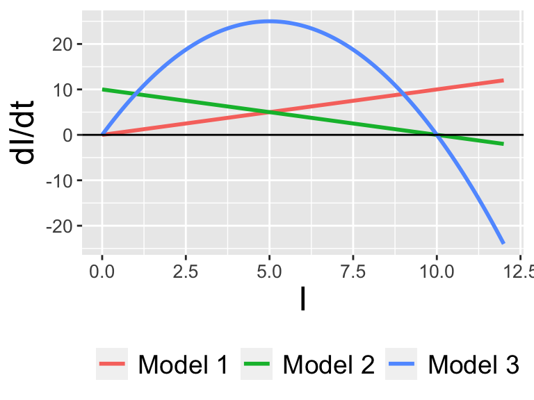
Figure 1.4: Comparing rates of change for three models
Figure 1.4 has a lot to unpack, but we can use some of our understanding of rates of change in calculus to compare the three models. Notice how the sign of \(\displaystyle \frac{dI}{dt}\) is always positive for Model 1, indicating that the solution (\(I\)) is always increasing. For Models 2 and 3, \(\displaystyle \frac{dI}{dt}\) equals zero when \(I=10\), which also is the value for \(N\) After that case, \(\displaystyle \frac{dI}{dt}\) turns negative, meaning that \(I\) is decreasing.
In summary, examining the graphs of the rates can tell a lot about the qualitative behavior of a solution to a differential equation even without the solution.
You may be used to working with algebraic equations (e.g. solve \(x^{2}-4=0\) for \(x\)) rather than differential equations. For algebraic equations the solution can be points (for our example, \(x=\pm2\)).↩︎
The COVID-19 pandemic that began in 2020 is an example of the heroic efforts of public health officials.↩︎