23.1 Random walk on a number line
The conceptual idea of a random walk begins on a number line. Let’s begin at the origin (so at \(t=0\) then \(x=0\)). Based on this number line we can only to the left or the right, with equal probability. At a given time we decide to move in a direction based on a random number \(r\) drawn between 0 and 1 (in R we do this with the command runif(1)). Figure 23.1 conceptually illustrates this random walk

Figure 23.1: Schematic diagram for one-dimensional random walk.
For each iteration of this process we will draw a random number using runif(1). We can code this process using a for loop:
### Number of steps our random walk takes
number_steps <- 100

### Set up vector of results
x <- array(0, dim = number_steps)

for (i in 2:number_steps) {
  if (runif(1) < 0.5) {
    x[i] <- x[i - 1] - 1
  } # Move right
  else {
    x[i] <- x[i - 1] + 1
  } # Move left
}

# Let's take a peek at our result:

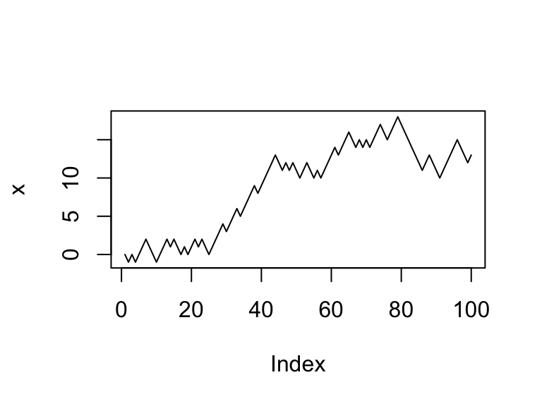
plot(x, type = "l")
print(mean(x)) # Where our average position was over the time interval## [1] 8.84print(sd(x)) # Where our standard deviation was over the time interval## [1] 5.807901Let’s remind ourselves what this code does:
number_steps <- 100: The number of times we draw a random number, referred to steps.x <- array(0,dim=number_steps): We are going to pre-allocate a vector (array) of our results. Values in this array are all set at 0 for convenience.- The for loop starts at the second step and then either adds or subtracts one from the prevoius position
x[i-1]and updates the result tox[i]. plot(x,type='l')makes a simple line plot of the results.
Now that you have run this code, try running it again. Do you get the same result? I hope you didn’t - because this process is random! It is interesting to run it several times because there can be a wide variance in our results - for some realizations of the sample path, we end up being strictly positive, other times we go negative, and other times we just hover around the middle.