10.5 Bayes’ Rule and Linear Regression

Returning back to our linear regression problem ($y=bx$). We have the following assumptions:

The data are independent, identically distributed. We can then write the likelihood function as the following: \[\begin{equation} \mbox{Pr}(\vec{y} | b) = \left( \frac{1}{\sqrt{2 \pi}}\right)^{4} e^{-\frac{(3-b)^{2}}{\sigma}} \cdot e^{-\frac{(5-2b)^{2}}{\sigma}} \cdot e^{-\frac{(4-4b)^{2}}{\sigma}} \cdot e^{-\frac{(10-4b)^{2}}{\sigma}} \end{equation}\]
Prior knowledge expects us to say that $b$ is normally distributed with mean 1.3 and standard deviation 0.1. Incorporating this information allows us to write the following: \[\begin{equation} \mbox{Pr}(b) =\frac{1}{\sqrt{2 \pi} \cdot 0.1} e^{-\frac{(b-1.3)^{2}}{2 \cdot 0.1^{2}}} \end{equation}\]

So when we combine the two pieces of information, the probability of the $b$, given the data $\vec{y}$ is the following:

\[\begin{equation} \mbox{Pr}(b | \vec{y}) \approx e^{-\frac{(3-b)^{2}}{2}} \cdot e^{-\frac{(5-2b)^{2}}{2}} \cdot e^{-\frac{(4-4b)^{2}}{2}} \cdot e^{-\frac{(10-4b)^{2}}{2}} \cdot e^{-\frac{(b-1.3)^{2}}{2 \cdot 0.1^{2}}} \tag{10.7} \end{equation}\]

Notice we are ignoring the terms $\displaystyle \left( \frac{1}{\sqrt{2 \pi}}\right)^{4}$ and $\displaystyle \frac{1}{\sqrt{2 \pi} \cdot 0.1}$, because per our discussion above not including them the does not change the location of the optimum value, only the value of the likelihood function. The plot of $\mbox{Pr}(b | \vec{y})$, assuming $\sigma = 1$ is shown in Figure 10.4:

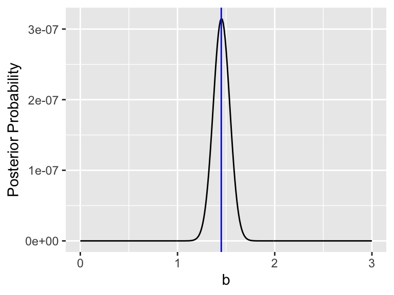
$Equation \@ref(eq:likelihood-bayes-10) with optimum value denoted in blue.$

Figure 10.4: Equation (10.7) with optimum value denoted in blue.

It looks like the value that optimizes our posterior probability is $b=$ 1.45. This is very close to the value of $\tilde{b}$ from the cost function approach. Again, this is no coincidence. Adding in prior information to the cost function or using Bayes’ Rule are equivalent approaches. Now that we have seen the usefulness of cost functions and Bayes’ Rule we can begin to apply this to larger problems involving more equations and data. In order to do that we need to explore some computational methods to scale this problem up - which we will do so in the next sections.