14.4 Exercises
global_temperature and for a linear, quadratic, cubic, and quartic polynomial and compute the BIC. What is the best approximating polynomial for the BIC? How does that compare to the best approximating model with the AIC?
&nsbp;
Exercise 14.2 You are investigating different models for the growth of a yeast species in population where \(V\) is the rate of reaction and \(s\) is the added substrate:
\[\begin{equation*} \begin{split} \mbox{Model 1: } & V = \frac{V_{max} s}{s+K_{m}} \\ \mbox{Model 2: } & V = \frac{K}{1+e^{-a-bs}} \\ \mbox{Model 3: } & V= K + Ae^{-bs} \end{split} \end{equation*}\]
With a dataset of 7 observations you found that the log-likelihood for Model 126.426, for Model 2 the log-likelihood is 15.587, and for Model 3 the the log-likelihood is 21.537. Apply the AIC and the BIC to evaluate which model is the best approximating model.
Exercise 14.3 An equation that relates a consumer’s nutrient content (denoted as \(y\)) to the nutrient content of food (denoted as \(x\)) is given by: \(\displaystyle y = c x^{1/\theta},\) where \(\theta \geq 1\) and \(c\) are both constants is a constant. We can apply linear regression to the dataset \((x, \; \ln(y) )\), so the intercept of the linear regression equals \(\ln(c)\) and the slope equals \(1 / \theta\).
- Show that you can write this equation as linear equation by applying a logarithm to both sides and simplifying.
- With the dataset
phosphorous, take the logarithim thedaphniavariable and then to determine a linear regression fit for your new linear equation. What are the reported values of the slope and intercept from the linear regression, and by association, \(c\) and \(\theta\)? - Use the function
logLikto report the likelihood of the fit. - What are the reported values of the AIC and the BIC?
- An alternative linear model is the equation \(y = a + b \sqrt{x}\). Use the R command
model2 <- lm(daphnia~I(sqrt(algae),data = phosphorous))to first obtain a linear fit. Then compute the log likelihood and the AIC and the BIC. Of the two models, which one is the better approximating model?
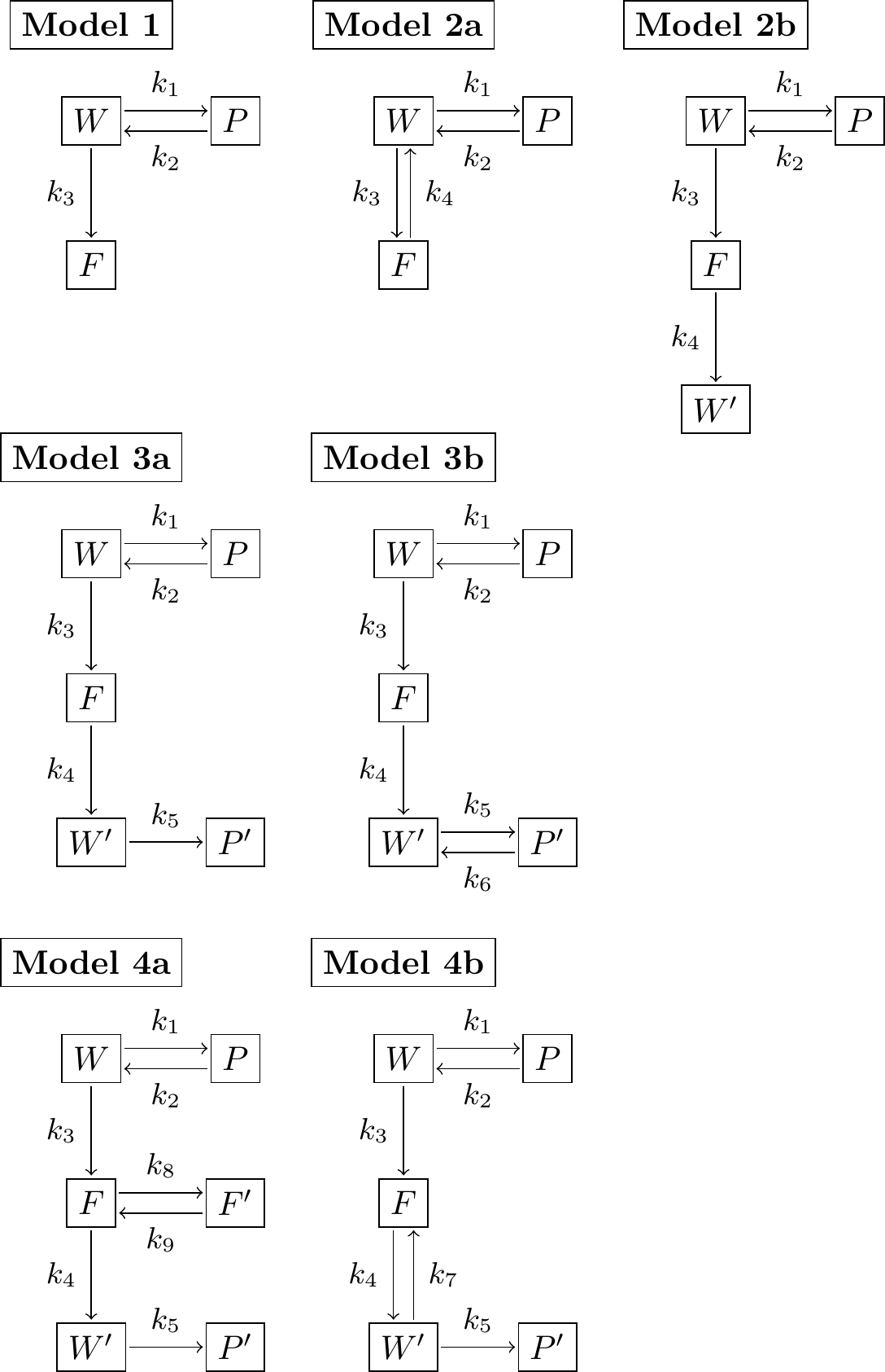
Figure 14.2: Reaction schemes.
Exercise 14.4 (Inspired by Burnham and Anderson (2002)) You are tasked with the job of investigating the effect of a pesticide on water quality, in terms of its effects on the health of the plants and fish in the ecosystem. Different models can be created that investigate the effect of the pesticide. Different types of reaction schemes for this system are shown in Figure 14.2, where \(F\) represents the amount of pesticide in the fish, \(W\) the amount of pesticide in the water, and \(S\) the amount of pesticide in the soil. The prime (e.g. \(F'\), \(W'\), and \(S'\) represent other bound forms of the respective state). In all seven different models can be derived.
These models were applied to a dataset with 36 measurements of the water, fish, and plants. The table for the log-likelihood for each model is shown below:
| Model | Log Likelihood |
|---|---|
| 1 | -90.105 |
| 2a | -71.986 |
| 2b | -56.869 |
| 3a | -31.598 |
| 3b | -31.563 |
| 4a | -8.770 |
| 4b | -14.238 |
- Use Figure to identify the number of parameters for each model.
- Apply the AIC and the BIC to the data in the above table to determine which is the best approximating model.