25.2 The Euler-Maruyama Method

The Euler-Maruyama method is a variation of Euler’s method that accounts for stochasticity and implements the random walk. We are going to build this up step by step.

First we write the $dx$ term as a difference equation: $dx = x_{n+1}-x_{n}$, where $n$ is the current step of Euler’s method. Likewise $dW(t) = W_{n+1} - W_{n}$, which represents one step of the random walk. We will approximate $W_{n+1}-W_{n} = \sqrt{\Delta t} Z_{1}$, where $Z_{1}$ is a random number from the standard unit normal distribution (done in R as rnorm(1)) and $\Delta t$ is the timestep length. When we put these together we have the following iterative method:

Given $\Delta t$ and starting value $x_{0}$,
Then compute the next step: $\displaystyle x_{1} = x_{0} + rx_{0} \left(1 - \frac{x_{0}}{K} \right) \; \Delta t + \sqrt{\Delta t} \; Z_{1}$
Repeat to step $n$: $\displaystyle x_{1} = x_{0} + rx_{0} \left(1 - \frac{x_{0}}{K} \right) \; \Delta t + \sqrt{\Delta t} \; Z_{1}$

That is it! We can apply this numerical method for as many steps as we want. I have some defined code that will apply the simulation, but just like euler or systems there are some things that need to be set first. In order to apply the Euler-Maruyama method you will need to define six things:

The size ($\Delta t$) of your timesteps.
The number of timesteps you wish to run the method. More timesteps means more computational time. If $N$ is the number of timesteps, $\Delta t \cdot N$ is the total time.
A function for our deterministic dynamics. For Equation (25.2) this equals $\displaystyle rx \left(1 - \frac{x}{K} \right)$.
A function for our stochastic dynamics. For Equation (25.2) this equals 1.
The values of the vector of parameters $\vec{\alpha}$. For the logistic differential equation we will take $r=0.8$ and $K=100$.
The standard deviation ($\sigma$) of our normal distribution and random walk. Typically this is set to 1, but can be varied if needed.

Sample code for this stochastic differential equation is shown below, with the resulting trajectory of the solution in Figure 25.1.

# Identify the deterministic and stochastic parts of the DE:
deterministic_logistic <- c(dx ~ r*x*(1-x/K))
stochastic_logistic <-  c(dx ~ 1)

# Identify the initial condition and any parameters
init_logistic <- c(x=3)  # Be sure you have enough conditions as you do variables. 
logistic_parameters <- c(r=0.8, K=100)   # parameters: a named vector

# Identify how long we run the simulation
deltaT_log <- .05    # timestep length
timeSteps_log <- 200   # must be a number greater than 1

# Identify the standard deviation of the stochastic noise
sigma_log <- 1

# Do one simulation of this differential equation
logistic_out <- euler_stochastic(deterministic_rate = deterministic_logistic,
                             stochastic_rate = stochastic_logistic,
                             init_cond = init_logistic,
                             parameters = logistic_parameters,
                             deltaT = deltaT_log,
                             n_steps = timeSteps_log,
                             sigma = sigma_log)

# Plot out the solution
ggplot(data = logistic_out) +
  geom_line(aes(x=t,y=x))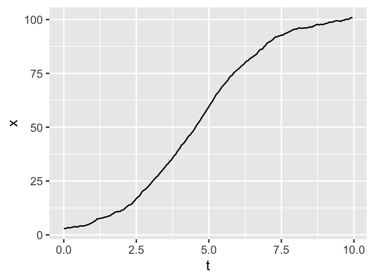

$One realization of Equation \@ref(eq:logistic-sde-25)$

Figure 25.1: One realization of Equation (25.1)

Let’s break this code down step by step:

We identify the deterministic and stochastic parts to our differential equation with the variables deterministic_logistic and stochastic_logistic. The same structure is used for Euler’s method from Section 4
Similar with Euler’s method we need to identify the initial conditions (init_logistic), parameters (logistic_parameters), $\Delta t$ (deltaT_log), and number of timesteps (timeSteps_log).
The standard deviation of the stochastic noise ($\sigma$) is represented with sigma_log.
The command euler_stochastic does one realization of the Euler-Maruyama method, returning a vector that we can then plot.

25.2.1 Multiple simulations

Figure 25.1 shows one sample trajectory of our solution. If you re-run this code several times and replot the solution you may see different trajectories plotted. In Section 22 we discussed the idea of stochastic simulation and how to re-run code several times and compute the ensemble average. We can put those ideas to good use here:

# Many solutions
n_sims <- 100  # The number of simulations

# Compute solutions
logistic_run <- rerun(n_sims) %>%
  set_names(paste0("sim", 1:n_sims)) %>%
  map(~ euler_stochastic(deterministic_rate = deterministic_logistic,
                             stochastic_rate = stochastic_logistic,
                             init_cond = init_logistic,
                             parameters = logistic_parameters,
                             deltaT = deltaT_log,
                             n_steps = timeSteps_log,
                             sigma = sigma_log)) %>%
  map_dfr(~ .x, .id = "simulation")


# Plot these all up together
  ggplot(data = logistic_run) +
  geom_line(aes(x=t, y=x, color = simulation)) +
  ggtitle("Spaghetti plot for the logistic SDE") +
  guides(color="none")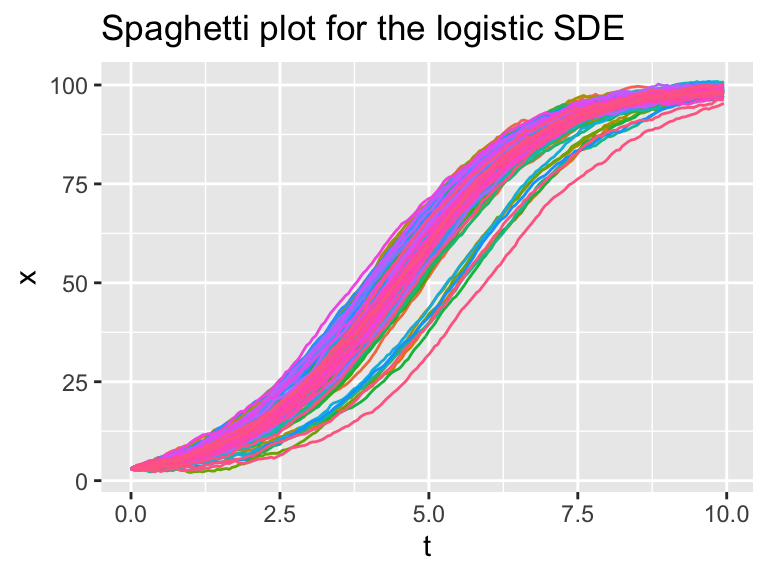

Figure 25.2: Several different realizations of the logistic SDE.

As you may recall, the main engine of the code is contained in the map( ~ euler_stochastic ... ) which re-runs the codes for the number of times specified in n_sims.

Figure 25.3 shows the ensemble average (median and 95% confidence interval) for the different simulations, recycling code from Section 22.

### Summarize the variables
summarized_logistic <- logistic_run %>%
  group_by(t) %>%  # All simulations will be grouped at the same timepoint.
  summarise(x = quantile(x, c(0.25, 0.5, 0.75)), q = c("q0.025", "q0.5", "q0.975")) %>%
  pivot_wider(names_from = q, values_from = x)

## `summarise()` has grouped output by 't'. You can override using the `.groups` argument.

### Make the plot
ggplot(data = summarized_logistic) +
  geom_line(aes(x = t, y = q0.5)) +
  geom_ribbon(aes(x=t,ymin=q0.025,ymax=q0.975),alpha=0.2) +
  ggtitle("Ensemble average plot for the logistic SDE")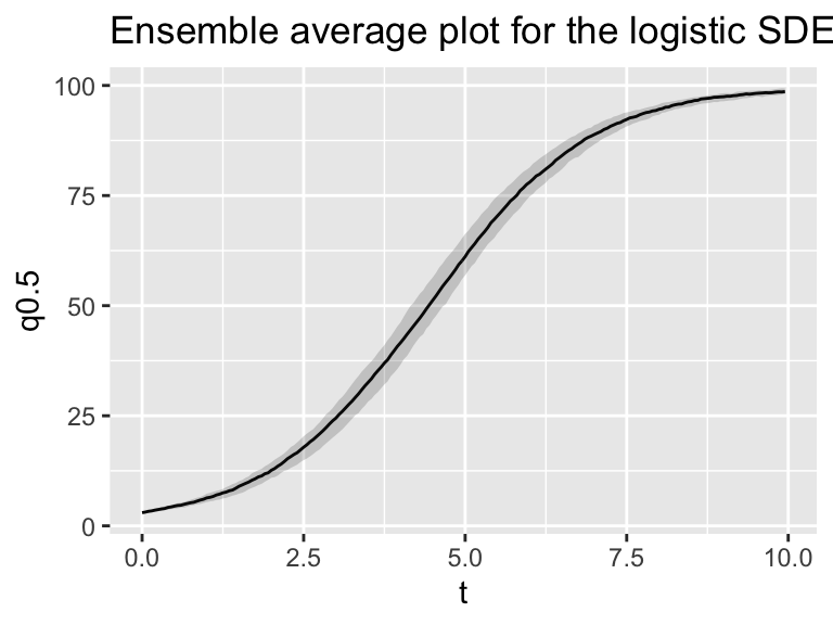

Figure 25.3: Ensemble average plot of the stochastic logistic SDE.

Breaking this code down, the variable summarized_logistic first groups the simulations by the variable t in order to compute the quantiles across each of the simulations. We then pivot resulting data frame in order to plot the ribbon.