12.2 Applying the likelihood to evaluate parameters

So with $p_{1}=65$ the modeled long-term trend seems to underestimate the data. Despite this, is the modeled growth with $p_{1}=65$ more plausible? We have nineteen measurements of the dog’s weight over time. Assuming these measures are all independent and identically distributed, we have the following likelihood function:

\[\begin{equation} L(p_{1}) = \prod_{i=1}^{19} \frac{1}{\sqrt{2 \pi} \sigma} e^{-\frac{(W_{i}-f(D_{i},p_{1}))^{2}}{2 \sigma^{2}}} \end{equation}\]

We can easily compute the associated likelihood values with the function compute_likelihood:

# Define the model we are using
my_model <- mass ~ p1 / (1 + exp(p2 - p3 * days))


# This allows for all the possible combinations of parameters
parameters <- tibble(p1 = c(78, 65), 
                     p2 = 2.461935, 
                     p3 = 0.017032
                     )

# Compute the likelihood and return the likelihood from the list
out_values <- compute_likelihood(my_model, wilson, parameters)$likelihood

# Return the likelihood from the list:
out_values

## # A tibble: 2 × 5
##      p1    p2     p3   l_hood log_lik
##   <dbl> <dbl>  <dbl>    <dbl> <lgl>  
## 1    78  2.46 0.0170 6.86e-29 FALSE  
## 2    65  2.46 0.0170 1.20e-27 FALSE

Hopefully this code seems familiar to you from Section 9. We made some modifications to streamline things:

We want to compare two values of p1, so when we defined parameters we included the two values of $p_{1}$ when defining parameters. The same values of p2 and p3 will apply to both. Don’t believe me? Type parameters at the console line to see!
Recall that when we apply compute_likelihood a list is returned (likelihood and opt_value . For this case we just want the likelihood data frame, hence the $likelihood at the end of compute_likelihood.

So we computed $L(78)$=6.8560765^{-29} and $L(65)$=1.2038829^{-27}. As you can see the value of $L(65)$ is a larger number compared to $p_{1}=78$. One way we can get a sense for the magnitude of the scale is by examining the ratio of the likelihoods:

\[\begin{equation} \mbox{ Likelihood ratio: } \frac{ L(p_{1}^{proposed}) }{ L(p_{1}^{current}) }, \end{equation}\]

So let’s compute this ratio: $\displaystyle \frac{ L(65) }{ L(78) }=$rround(out_values$l_hood[[2]]/out_values$l_hood[[1]])`. So with this comparison we would say that $p_{1}=65$ is more likely compared to the value of $p_{1}=78$.

Can we do better? What we can do is examine the likelihood ratio for another value. Since we might need to iterate through things let’s define a function that we can reuse:

# Define a function that computes the likelihood ratio for Wilson's weight
likelihood_ratio_wilson <- function(proposed, current) {

  # Define the model we are using
  my_model <- mass ~ p1 / (1 + exp(p2 - p3 * days))


  # This allows for all the possible combinations of parameters
  parameters <- tibble(p1 = c(current, proposed), p2 = 2.461935, p3 = 0.017032)

  # Compute the likelihood and return the likelihood from the list
  out_values <- compute_likelihood(my_model, wilson, parameters)$likelihood

  # Return the likelihood from the list:
  ll_ratio <- out_values$l_hood[[2]] / out_values$l_hood[[1]]

  return(ll_ratio)
}

# Test the function out:
likelihood_ratio_wilson(65, 78)

## [1] 17.55936

You should notice that the reported likelihood ratio matches up with our computation - yes! So let’s try to compute the likelihood ratio for $p_{1}=70$ compared to $p_{1}=65$. Try computing likelihood_ratio_wilson(70,65) - you should see that it is about 7.5 million times more likely!

I think we are onto something - Figure 12.4 compares the modeled values of Wilson’s weight for the different parameters:

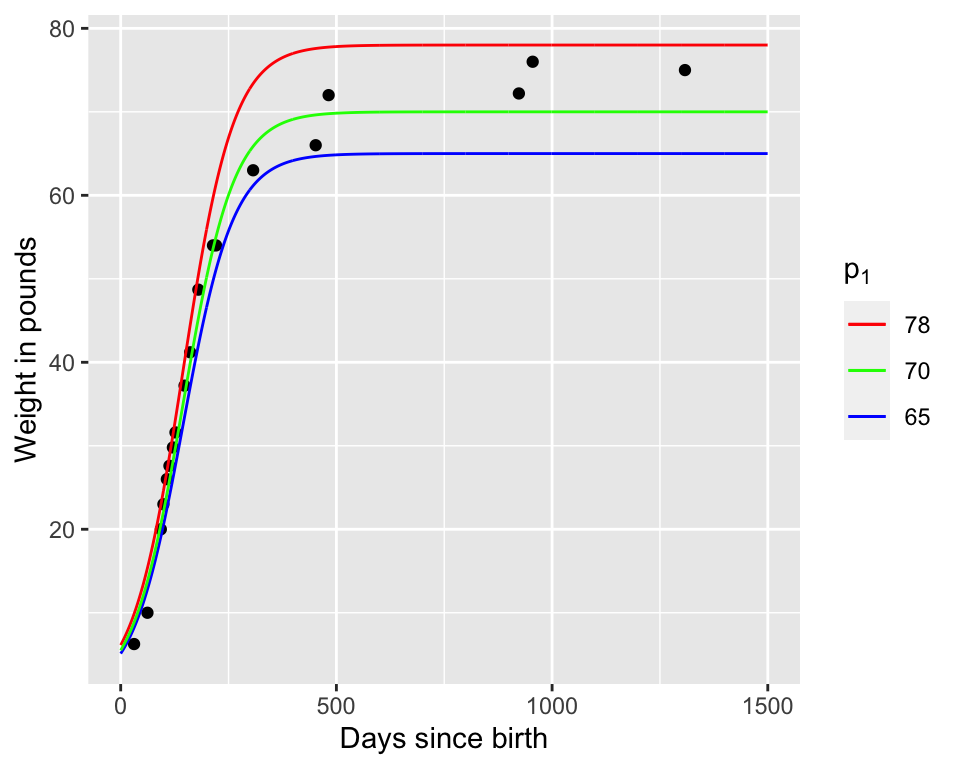
Figure 12.4: Comparison of our three estimates for Wilson’s weight over time.

So now, let’s try $p_{1}=74$ and compare the likelihoods: $\displaystyle \frac{ L(74) }{ L(70) }$=4.5897793^{-9}. This seems to be less likely because the ratio was significantly less than one. If we are doing a hunt for the best optimum value, then we would reject $p_{1}=74$ and keep moving on, perhaps selecting another value closer to 70.

However, the reality is a little different. For non-linear problems we want to be extra careful that we do not accept a parameter value that leads us to a local (not global) optimum. A way to avoid this is compare the likelihood ratio to a uniform random number $r$ between 0 and 1. We can do this very easily in R - remember the discussion of probability models in Section 9? At the R console type runif(1) - this creates one random number from the uniform distribution (remember the default range of the uniform distribution is $0 \leq p_{1} \leq 1$). The r in runif(1) stands for random. When I tried runif(1) I received a value of 0.126. Since the likelihood ratio is smaller than the random number we generated, we will reject the value of $p_{1}$ and try again, keeping 70 as our value.

The process keep the proposed value based on some decision metric is called a decision step.

12.2.1 An iterative method to estimate parameters

The neat part of the previous discussion is that we can automate this process, such as in the following table:

Iteration	Current value of $p_{1}$	Proposed value of $p_{1}$	$\displaystyle\frac{ L(p_{1}^{proposed}) }{ L(p_{1}^{current}) }$	Value of `runif(1)`	Accept proposed $p_{1}$?
0	78	NA	NA	NA	NA
1	78	65	17.55936	NA	yes
2	65	70	7465075	NA	yes
3	70	74	0.09985308	0.126	no
4	70	…	…	…	…

This table is the essence of what is called the Metropolis-Hastings algorithm. Here are the following components:

A defined likelihood function.
A starting value for your parameter.
A proposal value for your parameter.
Comparison of the likelihood ratios for the proposed to the current value ($\displaystyle \mbox{ Likelihood ratio: } \frac{ L(p_{1}^{proposed}) }{ L(p_{1}^{current}) }$). The goal of this algorithm method is to determine the parameter set that optimizes the likelihood function, or makes the likelihood ratio greater than unity. We will prefer values of $p_{1}$ that increase the likelihood.
A decision to accept the proposed parameter value. If the likelihood ratio is greater than 1, then we accept this value. However if the likelihood ratio is less than 1, we generate a random number $r$ (using runif(1)) and use this following process:

If $r$ is less than the likelihood ratio we accept (keep) the proposed parameter value.
If $r$ is greater than the likelihood ratio we reject the proposed parameter value.