3.1 Lynx and Hares
Our first example is a system of differential equations. The context is between the snowshoe hare and the Canadian lynx. Figure 3.1 shows a picture of them below from link
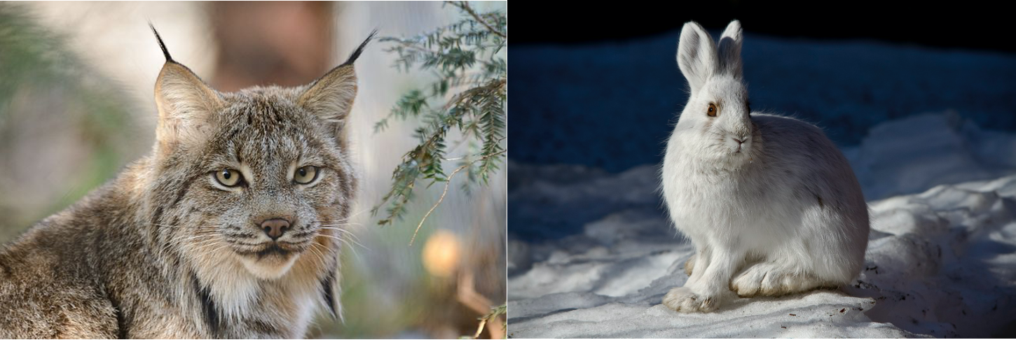
Figure 3.1: The lynx and hare - aren’t they beautiful?
Figure 3.2 timeseries of their population is shown with this figure from Stenseth et al. (1997).
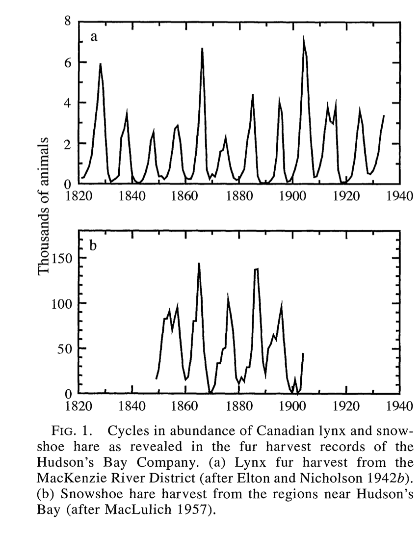
Figure 3.2: A timeseries of the combined lynx and hare system. Notice how the populations are coupled with each other.
Notice how in Figure 3.2 both populations seem to fluctuate periodically. One plausible reason is that the lynx prey on the snowshoe hares, which causes the population to initially decline. Once the snowshoe hare population declines, then there is less food for the lynx to survive, so their population declines. The decline in the lynx population causes the hare population to increase, and so on it goes …
In summary it is safe to say that the two populations are coupled to one another. But in order to understand how they are coupled together, first let’s consider the two populations separately.
The hares grow much more quickly than then lynx - in fact some hares have been known to reproduce several times a year. A reasonable assumption for large hare populations is that rate of change of the hares is proportional to the hare population. Based on this assumption Equation (3.1) describes the rate of change of the hare population, with \(H\) is the population of the hares:
\[\begin{equation} \frac{dH}{dt} = r H \tag{3.1} \end{equation}\]
In this case we know that the growth rate \(r\) is positive, so then the rate of change (\(H'\)) will be positive as well, and \(H\) will be increasing. Typical values given for \(r\) in Stenseth et al. (1997) are between 1.8 - 2.0 year\(^{-1}\). You may be thinking that the units on \(r\) seem odd - (year\(^{-1}\)). Another way to think about \(r\) is to take its inverse: \(r^{-1} \approx\) 0.5 - 0.55 years. Then \(r^{-1}\) represents the amount of time that passes before the hare population increases (pretty short!)
Let’s consider the lynx now. A approach is to assume their population declines exponentially, or changes at the rate proportional to the current population. Let’s consider \(L\) to be the lynx population, with the following differential equation (Equation (3.2)):
\[\begin{equation} \frac{dL}{dt} = -dL \tag{3.2} \end{equation}\]
We assume the death rate \(d\) in Equation (3.2) is positive, leading to a negative rate of change for the Lynx population (and a decreasing value for \(L\)). Typical values of \(d\) are 0.9 - 2.4 year\(^{-1}\). Similar to \(r\), another way to understand \(d\) is to take its inverse (about 0.4 - 1.1 years), which represents the amount of time that passes before the lynx population decreases by one.
The next part to consider is how the lynx and hare interact. Since the hares are prey for the lynx, when the lynx hunt, the hare population decreases. We can represent the process of hunting with the following adjustment to our hare equation:
\[\begin{equation} \frac{dH}{dt} = r H - b HL \end{equation}\]
So the parameter \(b\) represents the hunting rate. Notice how we have the term \(HL\) for this interaction. This term injects a sense of realism: if the lynx are not present (\(L=0\)), then the hare population can’t decrease due to hunting. We say that the interaction between the hares and the lynx with multiplication. Typical values for \(b\) are 480 - 870 hares \(\cdot\) lynx\(^{-1}\) year\(^{-1}\). It is okay if that unit seems a little odd to you - it should be! Here is one way to think about it. The quantity \(\displaystyle \frac{dH}{dt}\) represents the rate of change of the hares, so it should have units of hares per year. Since the term \(bHL\) has both lynx and hare, the units for \(b\) need to account for this.
How does hunting affect the lynx population? One possibility is that it increases the lynx population:
\[\begin{equation} \frac{dL}{dt} =bHL -dL \end{equation}\]
Notice the symmetry between the rate of change for the hares and the lynx equations. In many cases this makes sense - if you subtract a rate from one population, then that rate should be added to the receiving population. You could also argue that there is some efficiency loss in converting the hares to lynx - not all of the hare is converted into lynx biomass. In this situation we sometimes like to adjust the hunting term for the lynx equation with another parameter \(e\), representing the efficiency that hares are converted into lynx:
\[\begin{equation} \frac{dL}{dt} =e\cdot bHL -dL \end{equation}\]
(sometimes people just make a new parameter \(c=e \cdot b\), but for now we will just leave it as is). Equation (3.3) shows the coupled system of differential equations:
\[\begin{equation} \begin{split} \frac{dH}{dt} &= r H - b HL \\ \frac{dL}{dt} &=ebHL -dL \end{split} \tag{3.3} \end{equation}\]
The schematic diagram representing these interactions is the following is shown in Figure 3.3:
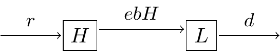
Figure 3.3: Schematic diagram Lynx-Hare system.
Equation (3.3) is a classical model in mathematical biology and differential equations - it is called the predator prey model, also known as the Lotka-Volterra equations. There is a lot of interesting mathematics from this system of equations that we will study later in this textbook. In later sections we will graphically and numerically analyze these equations and their solutions.