4.2 Building an iterative method
Now that we have worked on an example, let’s carefully formulate Euler’s method with another example. Consider the following equation that describes the rate of change of the spread of a disease (such as Ebola, as we covered in the first section):
\[ \frac{dI}{dt} = 0.003 I \cdot (4000-I) \]
Let’s call the function \(f(I) = 0.03 I\cdot (4000-I)\). In order to numerically approximate the solution, we will need to recall some concepts from calculus. One way that we can approximate the derivative is through a difference function:
\[ \frac{dI}{dt} = \lim_{\Delta t \rightarrow 0} \frac{I(t+\Delta t) - I(t)}{\Delta t} \]
As long as we consider the quantity \(\Delta t\) to be small (say for this problem 0.1 days if you would like to have units attached to this), we can approximate the derivative with difference function on the right hand side. With this information, we have a reasonable way to organize the problem:
\[\begin{align*} \frac{I(t+\Delta t) - I(t)}{\Delta t} &= 0.003 I \cdot (4000-I) \\ I(t+\Delta t) - I(t) &= 0.003 I \cdot (4000-I) \cdot \Delta t \\ I(t+\Delta t) &= I(t) + 0.003 I \cdot (4000-I) \cdot \Delta t \end{align*}\]
The last equation \(I(t+\Delta t) = I(t) + 0.03 I \cdot (4000-I) \cdot \Delta t = f(I) \cdot \Delta t\) is a reasonable way to define an iterative system, especially if we have a spreadsheet program. Here is some code in R that can define a for loop to do this iteratively and then plot the solution:
# Define your timestep and time vector
deltaT <- 0.1
t <- seq(0, 2, by = deltaT)

# Define the number of steps we take.  This is equal to 10 / dt (why?)
N <- length(t)

# Define the initial condition
i_approx <- 10

# Define a vector for your solution:the derivative equation
for (i in 2:N) { # We start this at 2 because the first value is 10
  didt <- .003 * i_approx[i - 1] * (4000 - i_approx[i - 1])
  i_approx[i] <- i_approx[i - 1] + didt * deltaT
}


# Define your data for the solution into a tibble:
solution_data <- tibble(
  time = t,
  infected = i_approx
)
Next we will plot our solution in Figure 4.2.
# Now plot your solution:
ggplot(data = solution_data) +
  geom_line(aes(x = time, y = infected)) +
labs(
  x = "Time",
  y = "Infected"
)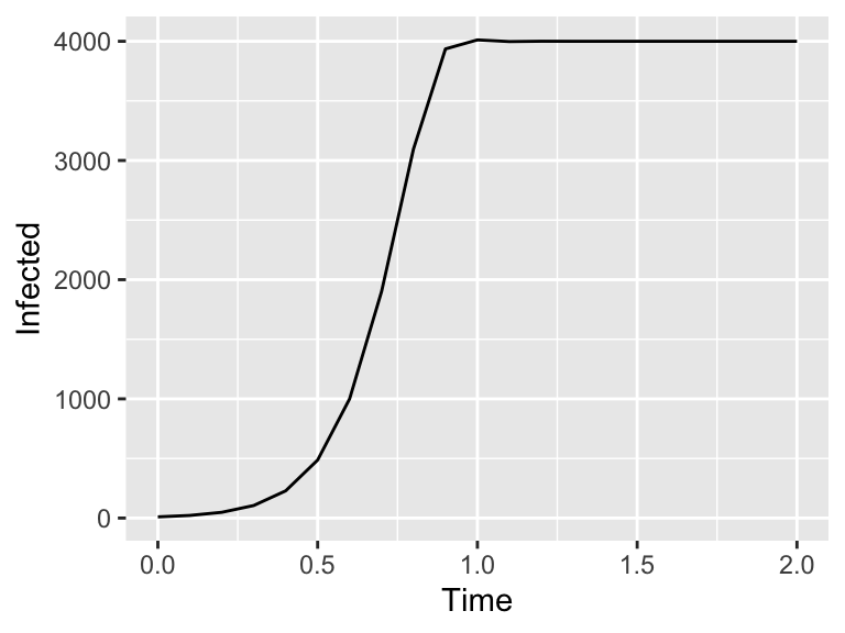
Figure 4.2: An iterative method
Ok, let’s break this code down step by step:
deltaT <- 0.1andt <- seq(0,2,by=deltaT)define the timesteps (\(\Delta t\)) and the output time vectort. We also defineN <- length(t)so we know how many steps we take.i_approx <- 10defines the initial condition to the system, in other words \(I(0)=10\).- The
forloop goes through this system - first computing the value of \(\displaystyle \frac{dI}{dt}\) and then forecasing out the next timestep \(I(t+\Delta t) = f(I) \cdot \Delta t\) - The remaining code plots the dataframe, like we learned in Section 2.
Let’s recap what we’ve learned to summarize Euler’s method. The most general form of a differential equation is:
\[ \displaystyle \frac{d\vec{y}}{dt} = f(\vec{y},\vec{\alpha},t), \] where \(\vec{y}\) is the vector of state variables you want to solve for, and \(\vec{\alpha}\) is your vector of parameters.
At a given initial condition, Euler’s method applies locally linear approximations to forecast the solution forward \(\Delta t\) time units:
\[ \vec{y}_{n+1} = y_{n} + f(\vec{y}_{n},\vec{\alpha},t_{n}) \cdot \Delta t \]
To generate Figure 4.2 we created the solution directly in R - but you don’t want to copy and paste the code. The demodeler package has a function called euler that does the same process to generate the output solution:
library(demodelr)

# Define the rate equation:
infection_eq <- c(didt ~ .003 * i * (4000 - i))

# Define the initial condition (as a named vector)
infection_init <- c(i = 10)

# Define deltaT and the time steps:
deltaT <- 0.2
n_steps <- 10

# Compute the solution via Euler's method:
out_solution <- euler(system_eq = infection_eq,
                      initial_condition = infection_init,
                      deltaT = deltaT,
                      n_steps = n_steps
                      )


# Now plot your solution:
ggplot(data = out_solution) +
  geom_line(aes(x = t, y = i)) +
labs(
  x = "Time",
  y = "Infected"
)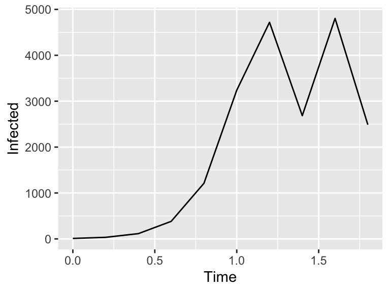
Figure 4.3: Euler's method solution
Let’s talk through the steps of this code as well:
- The line
infection_eq <- c(didt ~ .003 * i * (4000-i))represents the differential equation, written in formula notation. So \(\displaystyle \frac{dI}{dt} \rightarrow\)didtand \(f(I) \rightarrow\).003 * i * (4000-i)), with the variablei. - The initial condition \(I(0)=10\) is written as a named vector:
infection_init <- c(i=10). Make sure the name of the variable is consistent with your differential equation. - As before we need to identify \(\Delta t\) and the number of steps \(N\).
The command euler then computes the solution applying Euler’s method, returning a data frame so we can plot the results. Note the columns of the data frame are the variables \(t\) and \(i\) that have been named in our equations.