13.1 MCMC Parameter Estimation with an Empirical Model
Here are going to return to the problem exploring the phosphorous content in algae (denoted by \(x\)) to the phosphorous content in daphnia (denoted by \(y\)).
The equation we are going to fit is:
\[\begin{equation} y = c \cdot x^{1/\theta} \tag{13.1} \end{equation}\]
Equation (13.1) has two parameters \(c\) and \(\theta\), which range from \(0 \leq c \leq 2\) and \(1 \leq \theta \leq 20\), which we define below:
# Define the model
phos_model <- daphnia ~ c * algae^(1 / theta)

# Define the parameters that you will use with their bounds
phos_param <- tibble(
  name = c("c", "theta"),
  lower_bound = c(0, 1),
  upper_bound = c(2, 20)
)
The data that we use is the dataset phosphorous, which is already located in the demodelr package):
| algae | daphnia |
|---|---|
| 0.05376 | 1.08198 |
| 0.06506 | 1.13836 |
| 0.08217 | 1.26388 |
| 0.11031 | 1.43258 |
| 0.16061 | 1.45699 |
| 0.64414 | 1.51296 |
The final piece is to determine the number of iterations we run our the MCMC parameter estimate: That is it! All we need to do is to run our code:
# Define the number of iterations
phos_iter <- 1000

# Compute the mcmc estimate
phos_mcmc <- mcmc_estimate(
  model = phos_model,
  data = phosphorous,
  parameters = phos_param,
  iterations = phos_iter
)
The function mcmc_estimate may take some time (which is OK). This function has several inputs, which for convenience we write them on separate lines.
Let’s take a look at the data frame phosphorous_mcmc:
glimpse(phos_mcmc)## Rows: 1,000
## Columns: 4
## $ accept_flag <lgl> FALSE, FALSE, TRUE, FALSE, TRUE, TRUE, FALSE, FALSE, FALSE…
## $ l_hood <dbl> 16.4535871, 16.4535871, -5.3947728, -5.3947728, -0.9328032…
## $ c <dbl> 1.341311, 1.341311, 1.732444, 1.732444, 1.732444, 1.732444…
## $ theta <dbl> 7.722542, 7.722542, 7.722542, 7.722542, 11.421999, 7.40589…There are four columns here:
accept_flagtells you if at that particular iteration the MCMC estimate was accepted or not.l_hoodis the value of the likelihood for that given iteration.- The values of the parameters follow on the next few lines. Notice that \(\theta\) is written as
thetain the resulting data frame.
Next we need to visualize our results. The function mcmc_visualize summarizes and visualizes the results filtering on whenever accept_flag is TRUE (which means the parameter was accepted).
# Visualize the results
mcmc_visualize(
  model = phos_model,
  data = phosphorous,
  mcmc_out = phos_mcmc
)
## [1] "The parameter values at the optimized log likelihood:"
## # A tibble: 1 × 3
## l_hood c theta
## <dbl> <dbl> <dbl>
## 1 -5.56 1.65 8.98
## [1] "The 95% confidence intervals for the parameters:"
## # A tibble: 3 × 3
## probs c theta
## <chr> <dbl> <dbl>
## 1 2.5% 1.51 7.06
## 2 50% 1.60 10.8
## 3 97.5% 1.75 18.1## `stat_bin()` using `bins = 30`. Pick better value with `binwidth`.
## `stat_bin()` using `bins = 30`. Pick better value with `binwidth`.mcmc_visualize will generate output to the console that contains parameter statistics and confidence intervals. Additionally mcmc_visualize will produce different types of graphs. Let’s take a look at each one individually. The first plot is called a pairwise parameter plot. This contains a lot of different plots together, in a matrix pattern:
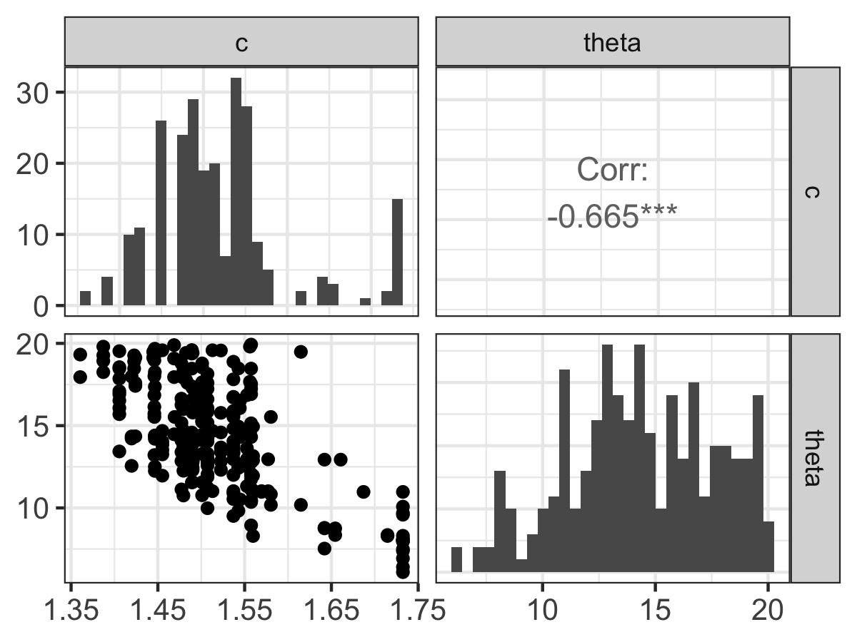
Figure 13.1: Pairwise parameter histogram from the MCMC parameter estimation for Equation (13.1).
Along of the diagonal of Figure 13.1 is a histogram of the accepted parameter values from the Metropolis algorithm. Depending on the results that you obtain, you may have some interesting shaped histograms. Generally they are grouped in the following ways:
- well-constrained: the parameter takes on a definite, well-defined value. The parameter \(c\) seems to behave like this.
- edge-hitting: the parameter seems to cluster near the edges of its value.
- non-informative: the histogram looks like a uniform distribution. The parameter \(\theta\) has some indications of being edge hitting, but we would need more iterations in order to determine this.
The off-diagonal terms in Figure 13.1 are interesting as well. The lower off-diagonal makes a scatter plot of the accepted values for the two parameters in the particular row and column, and the upper off-diagonal reports the correlation coefficient \(r\) of the variables in that particular row and column. The asterisks (*) denote the degree of significance of the linear correlation. Examining the pairwise parameter histogram helps ascertain the degree of equifinality in a particular set of variables (Beven and Freer 2001). In the Figure 13.1 it looks like c increases, \(\theta\) decreases. This degree of linear coupling means that we may not be able to independent resolve each parameter separately. The presence of equifinality does not mean the parameter estimation is a failure - just that we need to be aware of these relationships. Perhaps we may be able to go out in the field and measure a parameter more (for example \(c\)) more carefully, narrowing the range of accepted values.
Figure 13.2 displays an ensemble estimate of the results with the data. The ensemble average plot provides a high-level model-data overview. The black line represents the median ensemble average, and the grey is the 95% confidence interval, giving you a perspective of the model spread with the data. For our results here it does look there is wide variation in the model, most likely due to the relative wide confidence intervals on our parameters.
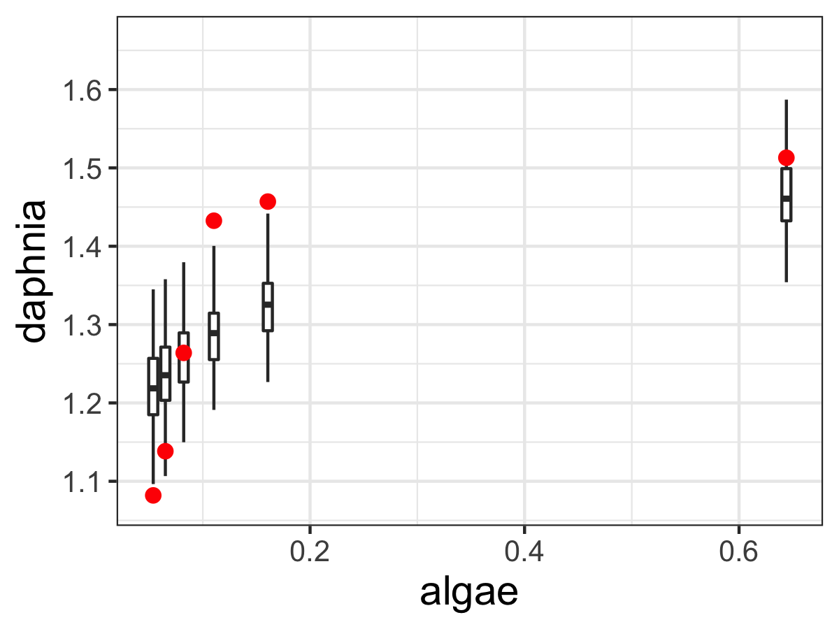
Figure 13.2: Ensemble output results from the MCMC parameter estimation for Equation (13.2).