22.3 Doing many simulations and visualizing

Now that we have some idea of a ensemble average, let’s put this into practice by doing some simulations of some one and two dimensional equations. What you will learn here is how to generate a simulation

For example consider the following code that produces a solution to the logistic differential equation:

logistic_eq <- c(dx ~ r * x * (1 - x / K)) # Define the rate equation

params <- c(r = .8, K = 100) # Identify any parameters

init_cond <- c(x = 3) # Initial condition
soln <- euler(
  system_eq = logistic_eq,
  initial_condition = init_cond,
  parameters = params,
  deltaT = .05,
  n_steps = 200
)

# Plot your solution:

ggplot() +
  geom_line(data = soln, aes(x = t, y = x)) +
  labs(
    x = "Time",
    y = "x"
  )

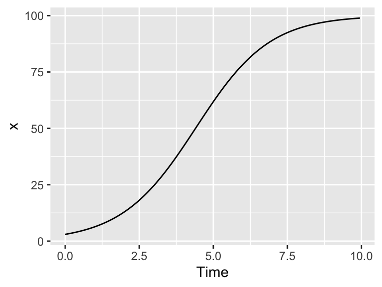
Figure 22.6: Solution to the logistic differential equation.

What if you wanted to investigate the effect of the initial condition on the solution, so the solution was randomly chosen, from a uniform distribution between 0 and 20? Well, to do one simluation is not a small modification of the code:

logistic_eq <- c(dx ~ r * x * (1 - x / K)) # Define the rate equation

params <- c(r = .8, K = 100) # Identify any parameters

init_cond_rand <- c(x = runif(1, min = 0, max = 20)) # Random initial condition

soln_rand <- euler(
  system_eq = logistic_eq,
  initial_condition = init_cond_rand,
  parameters = params,
  deltaT = .05,
  n_steps = 200
)

# Plot your solution:

ggplot() +
  geom_line(data = soln, aes(x = t, y = x), color = "black") +
  geom_line(data = soln_rand, aes(x = t, y = x), color = "red") +
  labs(
    x = "Time",
    y = "x"
  )

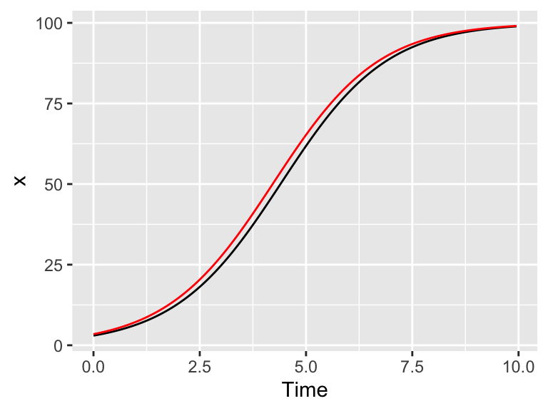
Figure 22.7: Solution to the logistic differential equation with a random initial condition (red). The original solution is also plotted for comparison.

Running several different iterations could quickly grow time consuming if you wanted to do this several times (think hundreds). Fortunately we will can use iteration here to compute and gather several different solutions. I am going to post the code and then we can deconstruct it:

n_sims <- 500 # The number of simulations

# Compute solutions
try1 <- rerun(n_sims, c(x = runif(1, min = 0, max = 20))) %>%
  set_names(paste0("sim", 1:n_sims)) %>%
  map(~ euler(
    system_eq = logistic_eq,
    initial_condition = .x,
    parameters = params,
    deltaT = .05,
    n_steps = 200
  )) %>%
  map_dfr(~.x, .id = "simulation")


# Plot these all up together
try1 %>%
  ggplot(aes(x = t, y = x)) +
  geom_line(aes(color = simulation)) +
  ggtitle("Random initial conditions") +
  guides(color = "none")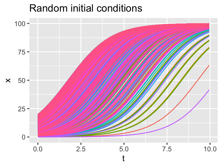

Figure 22.8: Many realiziations of the logistic differential equation with random initial conditions.

Wow! This plot is really interesting - it should show how even though the initial conditions vary between \(x=0\) to \(x=20\), eventually all solutions flow to the carrying capacity \(K=100\) (which is a stable equilbrium solution). Initial conditions that start closer to \(x=0\) take longer, mainly because they are so close to the other equilibrium solution at \(x=0\) (which is an unstable equilibrium solution).

Ok, let’s deconstruct this code line by line:

• rerun(n_sims, c(x=runif(1,min=0,max=20))) This line does two things: x=runif(1,min=0,max=20) makes a random initial condition, and the command rerun runs this again for n_sims times.
• set_names(paste0("sim", 1:n_sims)) This line distinguishes between all the different simulations.
• map(~ euler( ... ) You should be familiar with euler, but notice the pronoun .x that substitutes all the different initial conditions into Euler’s method. The map function iterates over each of the simulations.
• map_dfr(~ .x, .id = "simulation") This line binds everything up together.

This code applies a new concept called functional programming. This is a powerful tool that allows you to perform the process of iteration (do the same thing repeatedly) with uncluttered code. We won’t delve more into this here, but I encourage you to read about more programming concepts in https://r4ds.had.co.nz/iteration.html by Wickham and Grolemund