8.5 Nonlinear models

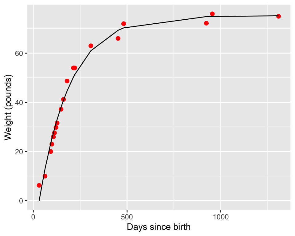
Many cases you will not be able to write your model in a linear format. You can still do a non-linear curve fit using the function nlm, however you will need to specify the function along with the formula you are using. For example if we try to fit the weight of the dog Wilson over time to the logistic equation we would have the following:

\[\begin{equation} W =f(D,a,b,c)= a - be^{ct}, \end{equation}\]

where we have the parameters \(a\), \(b\), and \(c\). Notice how \(W\) is a function of \(D\) and the parameters.

nonlinear_fit <- nls(mass ~ a - b * exp(c * days),
  data = wilson,
  start = list(a = 75, b = 30, c = -0.01)
)


summary(nonlinear_fit)

## 
## Formula: mass ~ a - b * exp(c * days)
## 
## Parameters:
##     Estimate Std. Error t value Pr(>|t|)    
## a 75.2349873  1.5726835   47.84  < 2e-16 ***
## b 90.7696994  3.3999731   26.70 1.07e-14 ***
## c -0.0060311  0.0004324  -13.95 2.26e-10 ***
## ---
## Signif. codes:  0 '***' 0.001 '**' 0.01 '*' 0.05 '.' 0.1 ' ' 1
## 
## Residual standard error: 2.961 on 16 degrees of freedom
## 
## Number of iterations to convergence: 11 
## Achieved convergence tolerance: 6.9e-06

The tricky part for a nonlinear model is that you need a starting value for the parameters (it is an iterative method). This can be tricky and takes some trial and error.

However once you have your fitted model, you can still plot the fitted values with the coefficients:

wilson_model <- broom::augment(nonlinear_fit, data = wilson)

ggplot(data = wilson) +
  geom_point(aes(x = days, y = mass),
    color = "red",
    size = 2
  ) +
  geom_line(
    data = wilson_model,
    aes(x = days, y = .fitted)
  ) +
  labs(
    x = "Days since birth",
    y = "Weight (pounds)"
  )

We will revisit these data later when we are making likelihood functions.