20.1 A series of equations
First let’s consider the differential equation \(\displaystyle \frac{dx}{dt} = 1-x^{2}\). This equation has an equibrium solution at \(x=\pm 1\). To classify the stability of the equilibrium solutions we apply the following test (developed in Section 5):
- If \(f'(y_{*})’>0\) at an equilibrium solution, the equilibrium solution \(y=y_{*}\) will be unstable.
- If \(f'(y_{*}) <0\) at an equilibrium solution, the equilibrium solution \(y=y_{*}\) will be stable.
- If \(f'(y_{*}) = 0\), we cannot conclude anything about the stability of \(y=y_{*}\).
Applying this test, we know \(f(x)=1-x^2\) and \(f'(x)=-2x\). Since \(f'(1)=-2\) and \(f'(-1)=2\), then the equilibrium solution \(x=1\) is stable and \(x=-1\) unstable.
Figure 20.1 shows a plot of the phase plane along with some solutions. Notice how the solutions seem to flow to \(x=1\) and away from \(x=-1\).
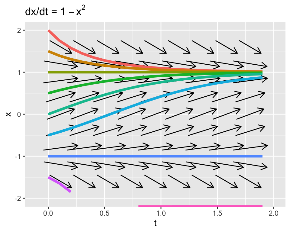
Figure 20.1: Phase plane of \(x'=1-x^{2}\)
Let’s modify and extend this example further. Consider two more differential equations:
- \(\displaystyle \frac{dx}{dt} = -1-x^{2}\): This differential equation does not have any equilibrium solutions, so we do not need to apply the stability test.
- \(\displaystyle \frac{dx}{dt} = -x^{2}\): The stability of the second equation is a little more tricky. While it has an equilibrium solution at \(x=0\), the stability test cannot apply because \(f'=-2x\) and \(f'(0)=0\). However investigating the sign of \(f(x)\) to the left and right of \(x=0\), we see that this solution is constantly decreasing, so the equilibrium is unstable.
So let’s also take a look at the phaseplanes for \(\displaystyle \frac{dx}{dt} = -1-x^{2}\) and \(\displaystyle \frac{dx}{dt} = -x^{2}\) along with the some solution curves (see also the accompanying figure).
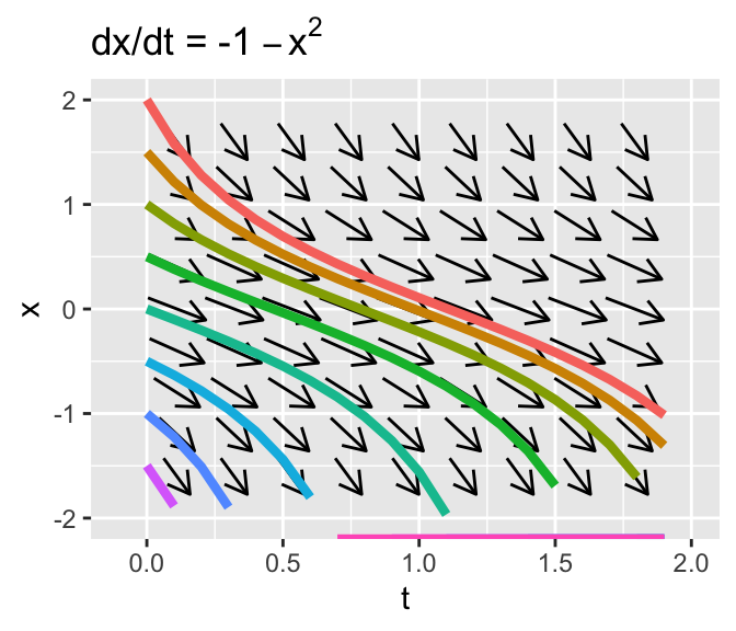
Figure 20.2: Phase plane of \(x'=-1-x^{2}\) and \(x'=-x^{2}\)
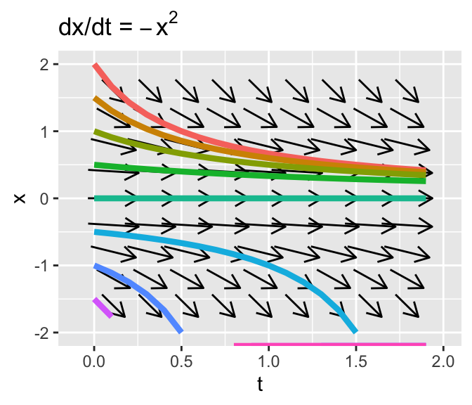
Figure 20.3: Phase plane of \(x'=-1-x^{2}\) and \(x'=-x^{2}\)
There is an interesting pattern going on here. Let’s build on these three examples in a more general context. Consider the differential equation \(\displaystyle \frac{dx}{dt} = c-x^{2}\). In our first example, \(c=1\). In the second example, \(c=-1\), and the third example \(c=0\). The phaseplanes from these examples illustrates how the value of \(c\) influences the phase line and the resulting solution.
Steady states to \(\displaystyle \frac{dx}{dt} = c-x^{2}\) are at \(x^{*}=\pm \sqrt{c}\). We can also test out the stability of our steady states using the stability test, with \(f(x)=c-x^{2}\) and \(f'(x)=-2x\):
- If \(c>0\) we have two steady states, summarized in the following table:
| Equilibrium solution | \(f'(x^{*})\) | Tendency of solution |
|---|---|---|
| \(x^{*}=\sqrt{c}\) | \(-2 \sqrt{c}\) | Stable |
| \(x^{*}=-\sqrt{c}\) | \(2 \sqrt{c}\) | Unstable |
(You should verify that the stability result we initially found when \(c=1\) matches the table.)
- If \(c=0\) there is only one steady state, summarized, in the following table:
| Equilibrium solution | \(f'(x^{*})\) | Tendency of solution |
|---|---|---|
| \(x^{*}=0\) | 0 | Inconclusive |
Based on the phaseplane for \(x'=-x^{2}\), the equilibrium solution \(x^{*}=0\) is unstable. If the initial condition \(x(0)\) is greater than 0, the solution flows towards \(x=0\), but if the initial condition is less than zero, the solution flows away from \(x=0\). This is similar to a one-dimensional analogue to a saddle node from Section 19.
- Finally, if \(c<0\), then there are no steady states because \(\sqrt{c}\) is does not have a real solution when \(c<0\). (Note: eigenvalues can be imaginary, but equilibrium solutions for our contexts can only be real). We can also test out the stability of our steady states using the stability test, with \(f(x)=c-x^{2}\) and \(f'(x)=-2x\):
Notice how different values of \(c\) influence both the value \((x^{*}=\pm \sqrt{c})\) and the stability of the equilibrium solution. Rather than making a series of tables, we can represent the dependence of the equilibrium solution and its stability in what is called a bifurcation diagram (Figure 20.4).
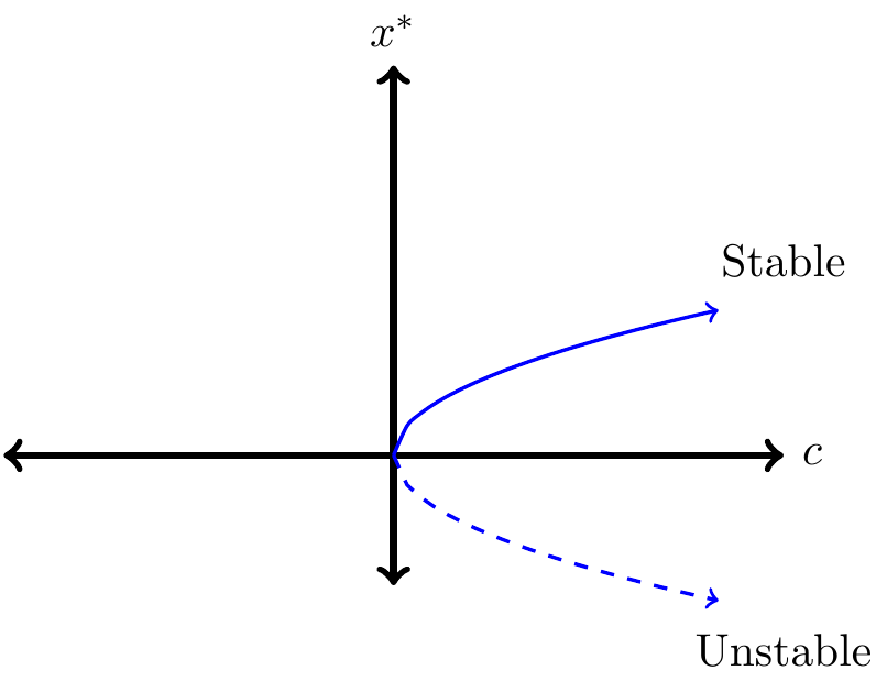
Figure 20.4: A saddle-node bifurcation
Let’s talk about Figure 20.4. The graph represents the value of the equilibrium solution (\(x^{*}\), vertical axis) as a function of the parameter \(c\) (horizontal axis). Since equilibrium solutions are characterized by \(x^{*}=\pm \sqrt{c}\) we have the “sideways parabola,” traced in blue in Figure 20.4. When \(c<0\), there is no equilibrium solution, (so nothing is plotted in the second and third quadrants of Figure 20.4). The difference between the solid and dashed lines in Figure 20.4 is used to distinguish between a stable equilibrium solution (\(x^{*}=\sqrt{c}\) when \(c>0\)) and unstable equilibrium solution (\(x^{*}=-\sqrt{c}\) when \(c>0\)). That is so cool that all the information about the equilibrium solution and its stability is contained in this diagram!
This particular example is called a saddle-node bifurcation. It might be helpful to think of this \(c\) like a tuning knob. As \(c>0\) we will always have two different equilibrium solutions that are symmetrical based on the value of \(c\). The positive one will be stable, the other unstable. As \(c\) gets smaller these equilbrium solutions will collapse into one, which will be unstable. If \(c\) is negative, the equilibrium solution disappears.