22.2 Computing ensemble averages

Let’s build up how to compute an ensemble average step by step. For example let’s say we have the following data in Table 22.1. Notice how all the simulations (sim1, sim2, sim3) share the variable t in common, so it makes sense to plot them on the same axis in Figure 22.3. We call a plot of all of the simulations together a spaghetti plot, because it can look like a bowl of spaghetti noodles was dumped all over the plot.

Table 22.1: Simulations of a variable at different times.

t	sim1	sim2	sim3
1	3.92	2.32	0.26
2	0.81	0.22	4.28
3	1.59	3.51	3.14
4	4.23	2.41	1.11
5	4.29	2.33	2.26

my_table %>%
  ggplot() +
  geom_point(aes(x = t, y = sim1)) +
  geom_line(aes(x = t, y = sim1)) +
  geom_point(aes(x = t, y = sim2)) +
  geom_line(aes(x = t, y = sim2)) +
  geom_point(aes(x = t, y = sim3)) +
  geom_line(aes(x = t, y = sim3)) +
  labs(x = "Time", y = "Simulation Value")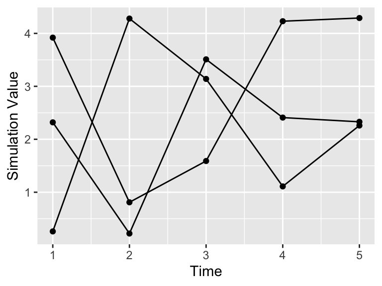

Figure 22.2: Initial Timeseries plot of the three simulations from Table 22.1.

One thing to adjust in the code used to produce the spaghetti plot in Figure 22.2 is that the code is really long - we needed a geom_point and geom_line for each simulation. While this isn’t bad when you have three simulations, one lesson we will learn is that the more simulations gives you better confidence in your results. If we have 500 simulations this would be a pain to code! Fortunately there is a command called pivot_longer that gathers different columns together (Table 22.2.

my_table_long <- my_table %>%
  pivot_longer(cols = c("sim1":"sim3"), names_to = "name", values_to = "value")

Table 22.2: Simulations of a variable at different times, condensed into a long table.

t	name	value
1	sim1	3.92
1	sim2	2.32
1	sim3	0.26
2	sim1	0.81
2	sim2	0.22
2	sim3	4.28
3	sim1	1.59
3	sim2	3.51
3	sim3	3.14
4	sim1	4.23
4	sim2	2.41
4	sim3	1.11
5	sim1	4.29
5	sim2	2.33
5	sim3	2.26

Notice how the command pivot_longer takes the different simulations (sim1, sim2, sim3) and reassigns the column names to a new column name and the values in the different columns to value. This process called pivoting creates a new data frame, which is easier to generate the spaghetti plot.

my_table_long %>%
  ggplot(aes(x = t, y = value, group = name)) +
  geom_point() +
  geom_line() +
  labs(x = "Time", y = "Simulation Value")

Figure 22.3: Timeseries plot of the three simulations from the pivoted data frame.

22.2.1 Grouping

The next step after pivoting is to collect the time points at \(t=1\) together, \(t=2\) together, and so on. In each of these groups we then compute the mean (average). This process is called grouping and then applying a summarizing function to all the members in a particular group (which in this case is the mean). Here is the code to do that process with the data frame my_table_long:

summarized_table <- my_table_long %>%
  group_by(t) %>%
  summarize(mean_val = mean(value))

Table 22.3: Simulations of a variable at different times, along with the mean value (last column).

t	mean_val
1	2.166667
2	1.770000
3	2.746667
4	2.583333
5	2.960000

Let’s break this down.

• The command group_by(t) means collect similar time points together
• The next line computes the mean. The command summarize means to that we are going to create a new data frame column (labeled mean_val that is the mean of all the grouped times, from the value column.

We can add this mean value to our data (Figure 22.4), represented with a thick red line.

my_table_long %>%
  ggplot(aes(x = t, y = value, group = name)) +
  geom_point() +
  geom_line() +
  geom_line(data = summarized_table, aes(x = t, y = mean_val), color = "red", size = 2, inherit.aes = FALSE) +
  geom_point(data = summarized_table, aes(x = t, y = mean_val), color = "red", size = 2, inherit.aes = FALSE) +
  guides(color = "none") +
  labs(x = "Time", y = "Simulation Value")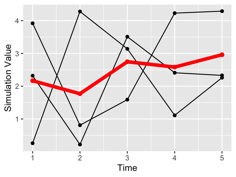

Figure 22.4: Timeseries plot of the three simulations.

Notice how we added the additional geom_point and geom_line with the option inherit.aes = FALSE. This stands for “inherit aesthetics” When you add a new data frame to a plot, the initial aesthetics (such as the color or the group) are passed on. Setting inherit.aes = FALSE allows you to work with a clean slate.

Computing the other parts of the ensemble average requires knowledge of how to compute percentiles of a distribution of values. For our purposes here we will use the 95% confidence interval, so that means the 2.5th, 97.5th percentile (which only 5% of the values will be outside of the specified interval), along with the median value (50th percentile). Let’s take a look at the code how do do that:

quantile_vals <- c(0.025, 0.5, 0.975)

quantile_table <- my_table_long %>%
  group_by(t) %>%
  summarize(
    q_val = quantile(value,
      probs = quantile_vals
    ),
    q_name = quantile_vals
  ) %>%
  pivot_wider(names_from = "q_name", values_from = "q_val", names_glue = "q{q_name}")

Table 22.4: Simulations of a variable at different times, along with the median and the 95% confidence interval.

t	q0.025	q0.5	q0.975
1	0.3630	2.32	3.8400
2	0.2495	0.81	4.1065
3	1.6675	3.14	3.4915
4	1.1750	2.41	4.1390
5	2.2635	2.33	4.1920

While this code is a little more involved, let’s break it down piece by piece:

• To make things easier the variable quantile_vals computes the different quantiles, expressed between 0 to 1 - so 2.5% is 0.025, 50% is 0.5, and 97.5% is .975.
• As above, we are still looking grouping by the variable t and summarizing our data frame.
• However rather than applying the mean, we are using the command quantile, whose value is computed with the new column q_val. Like the mean, we define which columns we apply the quantile function in the column value. We use probs = quantile_vals to specify the quantiles that we wish to compute.
• We also create a new column called q_name the contains the names of the quantile probabilities.
• The command pivot_wider takes the values in q_val with the associated names in q_name and creates new columns associated with each quantile. This process of making a data frame wider is the opposite of making a skinny and tall data frame with pivot_longer. Notice that a key convention in column names is that they don’t start with a number, so we glue a q onto the names of the column.

Wow. This is getting involved. One thing to keep in mind is that the the code as written should be easily adaptable if you need to compute an ensemble average. The last command about pivoting may seem foreign, but learning how to pivot data is a good skill to invest time in. If you take an introductory data science or data visualization course I bet you will learn more about the role of pivoting data - but for now you can just adapt the above code to your needs

Now onto plotting the data. What we will do is plot the ensemble average as a ribbon, so that is a new plot geom_ribbon. It requires a few more aesthetics (ymin and ymax, or the minimum and maximum y values to be plotted).

my_table_long %>%
  ggplot(aes(x = t, y = value, color = name)) +
  geom_point() +
  geom_line() +
  geom_line(data = quantile_table, aes(x = t, y = q0.5), color = "red", size = 2, inherit.aes = FALSE) +
  geom_point(data = quantile_table, aes(x = t, y = q0.5), color = "red", size = 2, inherit.aes = FALSE) +
  geom_ribbon(data = quantile_table, aes(x = t, ymin = q0.025, ymax = q0.975), alpha = 0.2, fill = "red", inherit.aes = FALSE) +
  guides(color = "none") +
  labs(x = "Time", y = "Simulation Value")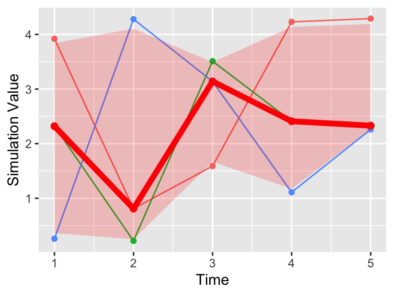

Figure 22.5: Timeseries plot of the three simulations, along with the 95% confidence interval (red).

A lot of this code to produce Figure 22.5 is similar to when we plotted the mean value (Figure 22.4), but we changed the second data frame to be plotted to quantile_table and included the geom_ribbon command. The command alpha = 0.2 refers to the transparency of the plot. The fill aesthetic just provides the shading (in other words the fill) between ymin and ymax.