10.1 Cost functions: likelihood functions in disguise
Another approach that can be incorporated into parameter estimation is the idea of a cost function. Let’s start again with the linear regression problem from Section 9:
Assume we have the following (limited) data set of points that we wish to fit a function of the form \(y=bx\) (note, we are forcing the intercept term to be zero).
| \(x\) | \(y\) |
|---|---|
| 1 | 3 |
| 2 | 5 |
| 4 | 4 |
| 4 | 10 |
Here, we will determine \(b\) through minimizing the square residual. We do this by computing the residual, or the expression \(y-bx\). Let’s extend out the above table a little more:
| \(x\) | \(y\) | \(bx\) | \(y-bx\) |
|---|---|---|---|
| 1 | 3 | \(b\) | \(3-b\) |
| 2 | 5 | \(2b\) | \(5-2b\) |
| 4 | 4 | \(4b\) | \(4-4b\) |
| 4 | 10 | \(4b\) | \(10-4b\) |
You can see how this residual changes \(y-bx\) for different values of \(b\):
| \(y-bx\) | \(b=1\) | \(b=3\) | \(b=-1\) |
|---|---|---|---|
| \(3-b\) | 2 | 0 | 4 |
| \(5-2b\) | 3 | -1 | 7 |
| \(4-4b\) | 0 | -8 | 8 |
| \(10-4b\) | 6 | -2 | 14 |
Notice that the values of the residual at each \((x,y)\) pair change as \(b\) changes - some of the residuals can be negative and some can be positive. If we were to assess the overall residuals as a function of the value of \(b\), we need to take into account not just the value of the residual (positive or negative), but rather the magnitude of the square residual. So for example, the square residual when \(b=1\) is:
\[\begin{equation} \mbox{ Square residual: } 2^{2}+3^{2}+0^{2}+6^{2} = 49 \end{equation}\]
The other square residuals are \(68\) when \(b=3\) and \(325\) when \(b=-1\). So of these choices for \(b\), the one that minimizes the square residual is \(b=1\).
Let’s generalize this to determine a function to compute the square residual for any value of \(b\). We will call this function \(S(b)\). How we do that is if we take the sum of the square difference (or the residual), we have:
\[\begin{equation} S(b)=(3-b)^2+(5-2b)^2+(4-4b)^2+(10-4b)^2 \tag{10.1} \end{equation}\]
This looks like a function of one variable. Let’s make a plot of \(S(b)\) in Figure 10.1. Notice how the plot of \(S(b)\) looks like a really nice quadratic function, with a minimum at \(b=1.86\). Did you notice that this value for \(b\) is the same value for the minimum that we found in the likelihood function from Section 9? In fact, if we multiplied out \(S(b)\) and collected terms, this would be a quadratic function - which has a well defined optimum value that you can find using calculus.
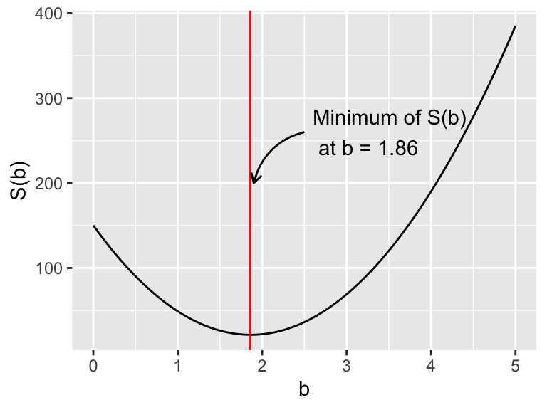
Figure 10.1: The square residual \(S(b)\). The vertical line denotes the minimum value at \(b=1.561\).
Let’s compare the value of \(b\) to the best fit line in Figure 10.2.
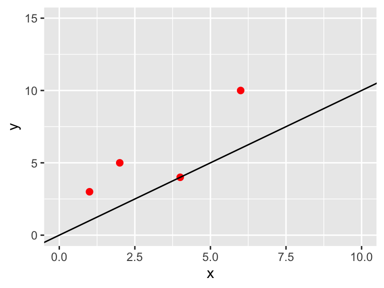
Figure 10.2: Data with the best fit line
The cost function approach described above seems to be working out well in that we have a value for \(b\), but it also looks like a lot of the data lies above the best fit line. We can address that later, but one approach is to include the uncertainty on each of the measured values in the cost function. The uncertainty may be the same (\(\sigma\)) for all measurements or it could vary from measurement to measurement. In both cases we divide each of the components of the cost function by the given uncertainty. We can represent this cost function more generally using \(\sum\) notation:
\[\begin{equation} S(\vec{\alpha}) = \sum_{i=1}^{N} \frac{(y_{i}-f(x,\vec{\alpha}))^{2}}{\sigma^{2}} \tag{10.2} \end{equation}\]
So examining Equation (10.1) to Equation (10.2) we have \(N=4\), \(\sigma = 1/\sqrt{2}\), and \(f(x_{i},\vec{\alpha} ) =bx\).