1.3 Model solutions

Let’s return back to possible solutions (in this case formulas for \(I(t)\)) for our models. Usually a differential equation also has a starting or an initial value (typically at \(t=0\)) that actualizes the solution. When we state a differential equation with a starting value we have an initial value problem. We will represent that initial value as \(I(0)=I_{0}\), where could be considered another parameter.

With that assumption, we can (and will solve later!) the following solutions for these models:

\[\begin{align*} \mbox{ Model 1 (Exponential): } & I(t) = I_{0}e^{kt} \\ \mbox{Model 2 (Saturating): } & I(t) = N-(N-I_{0})e^{-kt} \\ \mbox{Model 3 (Logistic): } & I(t) = \frac{N \cdot I_{0} }{I_{0}+(N-I_{0})e^{-kt}} \end{align*}\]

Notice how I assigned the names to each model (Exponential, Saturating, and Logistic). That may not mean much at the moment, but Figure 1.5 plots the three functions \(I(t)\) together when \(I_{0}=5\), \(k=0.03\), and \(N=4000\).

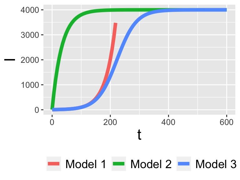
Figure 1.5: Three models compared

Notice how in Figure 1.5 Model 1 increases quickly - it actually grows without bound off the chart! Model 2 and Model 3 have saturating behavior, but it looks like Model 3 might be the one that actually captures the trend of the data.