15.2 The phase plane

The phase plane is helpful here to understand the nature of the equilibrium solution. Remember that the phase plane shows the motion of solutions, visualized as a vector. For the system we examined earlier let’s take a look at the phase plane. Here is some R code from the demodelr package to help you visualize a phaseplane:

# For a two variable systems of differential equations we need to define dx/dt and dy/dt separately:


systems_eq <- c(
  dxdt ~ 2 * x,
  dydt ~ x + y
)

# Now we plot the solution.
phaseplane(systems_eq, "x", "y")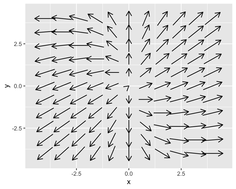

Let’s talk a little bit about each of the commands first.

You need to define both derivatives as separate functions (the lines that contain dxdt <- ... and dydt <- ...). We collect this in a vector called systems_eq, with the tilde (~) replacing the equals (=) sign.
The command phaseplane has required inputs of \(\displaystyle \frac{dx}{dt}\) and \(\displaystyle \frac{dy}{dt}\) and the names of the variables. There are additional inputs defining (1) the \(x\) and \(y\) windows (the default is \(-4 \leq x \leq 4\) and \(-4 \leq y \leq 4\)), and (2) the number of arrows in each row and column (default is 10). For example, the command phaseplane(systems_eq,'x','y',x_window=c(-5,5),y_window=c(-5,5),plot_points=20) will make a phaseplane diagram for the differential equation using 20 arrows with the axes limits to be between -5 and 5, and axis labels \(x\) and \(y\).

Notice how in the phaseline the arrows seem to spin out from the origin. We are going to discuss that below - but based on what we see we might expect the stability of the origin to be unstable.

15.2.1 What about one dimensional equations?

Remember how earlier on we had talked about equilibrium solutions with a phase line? It turns out we can use the command phaseplane to visualize a phase line. The subtlety is that we need to rewrite the one dimensional equation as a system of equations.

Let’s take the example \(\displaystyle \frac{dx}{dt} = -3x\)

# For a two variable systems of differential equations we need to define dx/dt and dy/dt separately:


systems_eq <- c(
  dt ~ 1,
  dx ~ -3 * x
)

# Now we plot the solution.
phaseplane(systems_eq, "t", "x")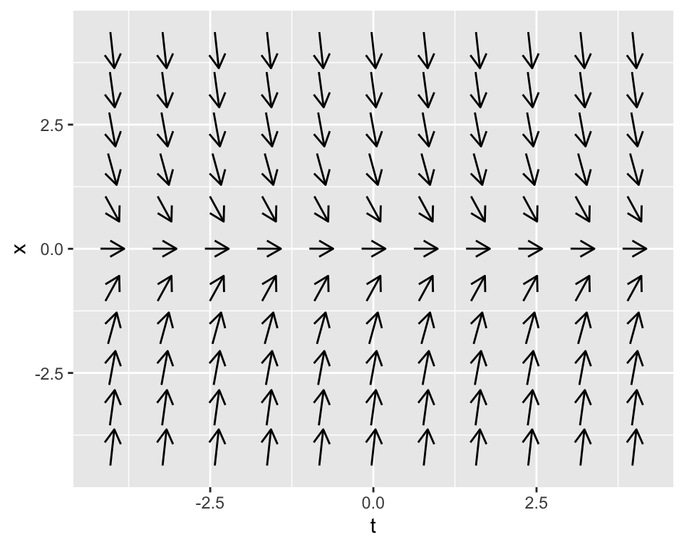

This codes looks similar to the previous example, with one small modification. For the variable systems_eq we need dt ~ 1 - which basically uses the horizontal axis as the time dependent variable - this basically says that the rate of change on the horizontal axis is constant (which yields the solution \(t\)). You will work out the details for converting a one-dimensional equation into a system of equations in Exercise 15.5.